22. Bioreactor Modeling: Governing Equations and Design Basis#
In this tutorial, we will learn how to design and model bioreactors for anaerobic, aerobic, and CO2/H2 gas-fed fermentations. We will first introduce the governing phenomenological equations (i.e., mass and energy balances, heat and mass transfer), then move into the following case studies, ordered by increasing complexity:
Anaerobic fermentation: conventional corn ethanol production.
Aerated fermentation: microbial oil production from sugar.
CO2/H2 gas-fed fermentation: acetic acid production from blast furnace steelmaking flue gas.
The goals of this tutorial are to:
Understand the governing equations and design basis of bioreactors in BioSTEAM.
Apply BioSTEAM unit operations to model different fermentation processes.
Understand the difference between anaerobic, aerobic, and gas-fed fermentations in terms of modeling complexity and economic impact.
22.1. Governing phenomenological equations#
There are 5 governing phenomenological equations that need to be satisfied in a bioreactor:
\(\mathrm{Conservation\ of\ mass}: ∑_{i\mathrm{\ \in\ products}} F_i - ∑_{i\mathrm{\ \in\ feeds}} F_i = ∑_i R_i\)
\(\mathrm{Phase\ equilibrium}: f^{gas}_i = f^{liq}_i\)
\(\mathrm{Conservation\ of\ energy}: \mathrm{Cooling\ Duty} = ∑_{i\mathrm{\ \in\ products}} H_i - ∑_{i\mathrm{\ \in\ feeds}} H_i\)
\(\mathrm{Mass\ transfer}: \mathrm{Gas\ Uptake\ Rate = Gas\ Transfer\ Rate}\)
\(\mathrm{Heat\ transfer}: \mathrm{Cooling\ Duty = Heat\ Transfer\ Rate}\)
\(F\) - Molar flow rate of an arbitrary chemical
\(f\) - Fugacity of an arbitrary chemical
\(R\) - Generation rate
\(H\) - Enthalpy flow rate
For a specific fermentation performance (e.g., titer and yield), we can solve for our mass and energy balances. This leaves us with the heat and mass transfer requirements, which must be satisfied by the detailed design of the bioreactor and its components (e.g., vessel, heat exchanger, compressor, agitator). Alternatively, given a specified design (e.g., vessel aspect ratio, agitation, gas flow rate), we could let the gas mass transfer rate dictate the fermentation performance.
In the following examples we will assume an experimentally verified fermentation performance and solve for the design of the bioreactor. As an exercise, we will first solve the problem manually with the help of BioSTEAM’s thermodynamic engine. Then, we will verify our results using BioSTEAM Unit Operations.
22.2. Corn ethanol anaerobic bioreactor#
In the conventional dry-grind process for corn ethanol production, the corn is first liquified and saccharified to create a slurry. This glucose is then fermented to ethanol and carbon dioxide using yeast:
\(\mathrm{Glucose \rightarrow 2\ Ethanol + 2\ CO_2}\)
We will assume the following fermentation performance:
Feed flow rate: 150,000 kg\(\cdot\)h\(^{-1}\)
Feed glucose concentration: 20% wt
Ethanol yield: 95% theoretical
Temperture: 32 \(^\circ\)C
[1]:
feed_flow = 150000
x_Glucose = 0.20
yield_EtOH = 0.95
T_operation = 32 + 273.15
22.2.1. Mass balance#
We can solve for the total product flow rates by reacting the feed assuming the given yield. Mathematically, this translates to:
\(F_{i,\ \mathrm{out}} = F_{i,\ \mathrm{in}} + C_i \cdot X_{\mathrm{Glucose}} \cdot F_{\mathrm{Glucose,\ in}}\)
\(X\) - Extent of reaction.
\(C\) - Stoichiometric reaction coefficient.
\(i\) - Index for an arbitrary chemical.
We can model the stoichiometric reaction using Reaction objects to “react” a stream.
To compute the flow rate of chemicals as they partition into the gas and liquid phases (i.e., the vent and effluent streams), we need to meet the vapor-liquid equilibrium criteria, which translates to the fugacity of each chemical in each phase must be the same.
\(f^\alpha_i = f^\beta_i\)
\(f^\alpha\) - Fugacity in phase \(\alpha\).
\(f^\beta\) - Fugacity in phase \(\beta\).
Phase equilibrium can be challenging to solve given how fugacity is a highly nonlinear and tightly coupled function of composition, temperature, and pressure. In BioSTEAM, we can quickly perform vapor-liquid equilibrium to partition the flows into the vent and effluent streams:
[2]:
import biosteam as bst; bst.nbtutorial()
from biosteam.units.design_tools import aeration

# Define chemicals
bst.settings.set_thermo(
    ['Water', 'Ethanol', 'Glucose', 'CO2', 'Yeast'],
    db='BioSTEAM'
)

# Create the feed
feed = bst.Stream(
    Water=1 - x_Glucose,
    Glucose=x_Glucose,
    total_flow=feed_flow,
    units='kg/hr',
    T=T_operation,
    P=101325,
)

# Create product streams
broth = bst.Stream()
vent = bst.Stream(phase='g')
product = bst.MultiStream.from_streams([vent, broth])

# Define the reaction
production = bst.Reaction(
    'Glucose -> 2 Ethanol + 2 CO2',
    X=yield_EtOH,
)
growth = bst.Reaction(
    'Glucose -> Yeast',
    X=yield_EtOH,
    correct_mass_balance=True,
)
fermentation = bst.ReactionSystem(production, growth)

# Convert the feed to product
broth.copy_like(feed)
fermentation(broth)

# Perform vapor-liquid equilibrium (uses Henry's constants).
# Using product.vle(T=T_operation, P=101325) also works, but less accurate for fermentation broths.
aeration.vent_broth(vent, broth)

feed.show('cwt')
print()
fermentation.show()
print()
product.show('cwt')
Stream: feed
phase: 'l', T: 305.15 K, P: 101325 Pa
flow (%): Water    80
          Glucose  20
          -------  1.5e+05 kg/hr

ReactionSystem:
[0]  Reaction (by mol):
     stoichiometry                 reactant    X[%]
     Glucose -> 2 Ethanol + 2 CO2  Glucose    95.00
[1]  Reaction (by mol):
     stoichiometry          reactant    X[%]
     Glucose -> 7.97 Yeast  Glucose    95.00

MultiStream:
phases: ('g', 'l'), T: 305.15 K, P: 101325 Pa
flow (%): (g) Water    1.38
              Ethanol  1.59
              CO2      97
              -------  1.42e+04 kg/hr
          (l) Water    88.2
              Ethanol  10.6
              Glucose  0.0552
              CO2      0.125
              Yeast    1.05
              -------  1.36e+05 kg/hr
22.2.2. Energy balance#
Now that we have solved the mass balance, we can estimate our cooling duty. The enthalpy flow rate of a stream depends on the temperature, pressure, and material flow rates. In BioSTEAM, we can estimate the enthalpy of a stream by using the Stream.H and Stream.Hf properties. Note that H does include
heats of formation at its reference state while Hf is just the heats of formation.
[3]:
cooling_duty = (product.Hf + product.H) - (feed.Hf + feed.H) # Enthalpy change (including heats of formation)
print('Cooling duty:', f'{cooling_duty:.3g}', 'kJ/hr')
Cooling duty: -1.37e+07 kJ/hr
22.2.3. Bioreactor sizing#
To size the bioreactor, we will need to make the following heurstic design specifications:
\(R\) - length to diameter: 3
\(V_{\mathrm{max}}\) - maximum reactor volume: 1000 m3
\(f\) - working volume: 90%
\(\tau_{\mathrm{reaction}}\) - reaction time: 60 h
\(\tau_{\mathrm{cleaning}}\) - clean up time: 3 h
\(\tau_{\mathrm{loading}}\) - loading time: 1 h
\(R\) - height to diameter ratio: 3
This allows us to solve for the reactor volume, number of reactors, and reactor dimensions:
\(V_{\mathrm{total}} = \nu(\tau_{\mathrm{reaction}} + \tau_{\mathrm{cleaning}} + \tau_{\mathrm{loading}}) \cdot f^{-1}\)
\(N_{\mathrm{reactors}} = \mathrm{ceil}(V_{\mathrm{total}} \cdot V_{\mathrm{max}^{-1}})\)
\(V_{\mathrm{reactor}} = V_{\mathrm{total}} N_{\mathrm{reactors}}^{-1}\)
\(D = (4 \pi V_{\mathrm{reactor}} R)^{1/3}\)
\(H = D \cdot R\)
\(\nu\) - Volumetric flow rate
\(N_{reactors}\) - Number of reactors
\(V_{total}\) - Total volume of all reactors
\(V_{reactor}\) - Volume of a reactor
\(D\) - Diameter
\(H\) - Height
[4]:
from math import ceil, pi as π

# Heuristic specifications
R = 3
V_max = 1000
f = 0.90
tau_reaction = 60
tau_cleanup = 3
tau_loading = 1

# Solve for number of reactors and the volume of an individual reactor
𝜈 = feed.F_vol
V_total = 𝜈 * (tau_reaction + tau_cleanup + tau_loading) / f
N_reactors = ceil(V_total / V_max)
V_reactor = V_total / N_reactors
print('Number of reactors:', N_reactors)
print('Reactor volume:', f"{V_reactor:.3g}", 'm3')

# Solve for the diameter and height
D = (4 * V_reactor / π / R)**(1/3)
H = D * R
print('Reactor height:', f"{H:.3g}", 'm')
print('Reactor diameter:', f"{D:.3g}", 'm')
Number of reactors: 11
Reactor volume: 913 m3
Reactor height: 21.9 m
Reactor diameter: 7.29 m
22.2.4. Heat exchange#
The most commonly used bioreactor heat exchanger configuration is the jacketed vessel. A full jacket provides a constant heat transfer area to the medium. In order to meet the cooling requirement, the flow rate of the cooling agent (e.g., chilled water) can be varied. The greater the flow rate, the greater the overall heat transfer coefficient, and the greater the driving force (i.e., the temperature difference across the jacket). Because the temperature of the utility changes across the jacket, we use the log-mean temperature difference as the driving force (LMTD).
\(Q = U A \Delta T_{\mathrm{LMTD}}\)
\(Q = F_{\mathrm{utility}} (h_\mathrm{utility,\ in} - h_\mathrm{utility,\ out})\)
\(\Delta T_{\mathrm{LMTD}} = (\Delta T_{\mathrm{in}}-\Delta T_{\mathrm{out}}) \ln(\Delta T_{\mathrm{in}} / \Delta T_{\mathrm{out}})^{-1}\)
\(\Delta T_{\mathrm{in}} = T_{\mathrm{utility,\ in}} - T_{\mathrm{operation}}\)
\(\Delta T_{\mathrm{out}} = T_{\mathrm{utility,\ out}} - T_{\mathrm{operation}}\)
\(U\) - Overall heat trasfer coefficient
\(Q\) - Cooling duty
\(T\) - Temperature
\(h\) - Specific molar enthalpy
Estimating the overall heat transfer coefficient can be challenging due to its dependence on detailed design of the bioreactor (e.g., agitation) and mixture properties (e.g., density, conductivity). As a preliminary estimate, we can assume that the temperature of the outlet utility is simply the maximum allowable temperature for smooth regeneration (chilled water cannot come back too hot to the cooler). Because the cost of chilled water usage is estimated based on the total heat transfered (not on the actual flow rate), this assumption does not impact our economic analysis.
[5]:
# Additional assumptions/specifications
T_utility_out = 27.22 + 273.15
T_utility_in = 7.22 + 273.15

# Solve for utility requirements
chilled_water_in = bst.Stream(Water=1, T=T_utility_in)
chilled_water_out = bst.Stream(Water=1, T=T_utility_out)
F_utility = cooling_duty / (chilled_water_in.h - chilled_water_out.h)

print('Chilled water flow rate:',  f'{F_utility:.3g}', 'kmol/hr')
Chilled water flow rate: 9.07e+03 kmol/hr
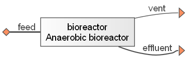
22.2.5. Standard anaerobic bioreactor model#
BioSTEAM streamlines the modeling, design, costing of bioreactors. Let’s use BioSTEAM’s AnaerobicBioreactor model to model the corn ethanol fermentation:
[6]:
import biosteam as bst; bst.nbtutorial()

bioreactor = bst.AnaerobicBioreactor(
    ins=feed,
    outs=('vent', 'effluent'),
    reactions=fermentation,
    T=T_operation,
    V_wf=f,
    V_max=V_max,
    tau=tau_reaction,
    tau_0=tau_cleanup,
    loading_time=tau_loading,
    length_to_diameter=R,
    heat_exchanger_configuration='jacketed',
)
bioreactor.simulate()
bioreactor.diagram(format='png')
bioreactor.show('cwt')
AnaerobicBioreactor: bioreactor
ins...
[0] feed
    phase: 'l', T: 305.15 K, P: 101325 Pa
    flow (%): Water    80
              Glucose  20
              -------  1.5e+05 kg/hr
outs...
[0] vent
    phase: 'g', T: 305.15 K, P: 101325 Pa
    flow (%): Water    1.38
              Ethanol  1.59
              CO2      97
              -------  1.42e+04 kg/hr
[1] effluent
    phase: 'l', T: 305.15 K, P: 101325 Pa
    flow (%): Water    88.2
              Ethanol  10.6
              Glucose  0.0552
              CO2      0.125
              Yeast    1.05
              -------  1.36e+05 kg/hr
[7]:
bioreactor.results(basis='SI')
[7]:
| Anaerobic bioreactor | Units | bioreactor | |
|---|---|---|---|
| Electricity | Power | kW | 90.4 |
| Cost | USD/hr | 7.07 | |
| Chilled water | Duty | kJ/hr | -1.37e+07 |
| Flow | kmol/hr | 9.17e+03 | |
| Cost | USD/hr | 68.4 | |
| Design | Reactor volume | m³ | 913 |
| Batch time | hr | 64 | |
| Loading time | hr | 1 | |
| Number of reactors | 11 | ||
| Residence time | hr | 60 | |
| Vessel type | Vertical | ||
| Length | m | 21.9 | |
| Diameter | m | 7.29 | |
| Weight | kg | 1.12e+05 | |
| Wall thickness | m | 0.0119 | |
| Jacketed diameter | m | 7.4 | |
| Vessel material | Stainless steel 316 | ||
| Purchase cost | Vertical pressure vessel (jacketed) (x11) | USD | 4.63e+06 |
| Platform and ladders (x11) | USD | 9.69e+05 | |
| Agitator - Agitator (x11) | USD | 1.77e+05 | |
| Total purchase cost | USD | 5.78e+06 | |
| Installed equipment cost | USD | 2.04e+07 | |
| Utility cost | USD/hr | 75.5 |
Note how all BioSTEAM results match our calculations.
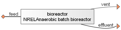
22.2.6. NREL anaerobic bioreactor model#
While modeling of mass and energy balances is standard, the design and costing of the anaerobic bioreactors may have different approaches in prelimiary techno-economic analysis. A report from NREL on cellulosic ethanol production offers cost correlations based on reactor volume and duty. Let’s use the NRELAnaerobicBioreactor model and have a look at how results may difer.
[8]:
bioreactor = bst.NRELAnaerobicBatchBioreactor(
    ins=feed,
    outs=('vent', 'effluent'),
    reactions=fermentation,
    T=T_operation,
    V_wf=f,
    V_max=V_max,
    tau=tau_reaction,
    tau_0=tau_cleanup,
    loading_time=tau_loading,
)
bioreactor.simulate()
bioreactor.diagram(format='png')
bioreactor.show('cwt')
NRELAnaerobicBatchBioreactor: bioreactor
ins...
[0] feed
    phase: 'l', T: 305.15 K, P: 101325 Pa
    flow (%): Water    80
              Glucose  20
              -------  1.5e+05 kg/hr
outs...
[0] vent
    phase: 'g', T: 305.15 K, P: 101325 Pa
    flow (%): Water    1.87
              Ethanol  2.16
              CO2      96
              -------  1.05e+04 kg/hr
[1] effluent
    phase: 'l', T: 305.15 K, P: 101325 Pa
    flow (%): Water    85.9
              Ethanol  10.3
              Glucose  0.0537
              CO2      2.79
              Yeast    1.02
              -------  1.4e+05 kg/hr
[9]:
bioreactor.results()
[9]:
| NRELAnaerobic batch bioreactor | Units | bioreactor | |
|---|---|---|---|
| Electricity | Power | kW | 117 |
| Cost | USD/hr | 9.13 | |
| Chilled water | Duty | kJ/hr | -1.45e+07 |
| Flow | kmol/hr | 9.69e+03 | |
| Cost | USD/hr | 72.3 | |
| Design | Reactor volume | m3 | 933 |
| Batch time | hr | 64 | |
| Loading time | hr | 1 | |
| Number of reactors | 11 | ||
| Recirculation flow rate | m3/hr | 13.1 | |
| Reactor duty | kJ/hr | -1.45e+07 | |
| Cleaning and unloading time | hr | 3 | |
| Working volume fraction | 0.9 | ||
| Purchase cost | Heat exchangers (x11) | USD | 2.21e+05 |
| Reactors (x11) | USD | 5.01e+06 | |
| Agitators (x11) | USD | 3.12e+05 | |
| Cleaning in place | USD | 1.98e+05 | |
| Recirculation pumps (x11) | USD | 1.37e+05 | |
| Total purchase cost | USD | 5.88e+06 | |
| Installed equipment cost | USD | 9.14e+06 | |
| Utility cost | USD/hr | 81.4 |
The NREL model has significantly lower capital. It is normal for equipment costs to vary this much, but they should be within the same order of magnitude. The main difference between the two methods is that the “standard” method is based on correlations of the average capital costs paid in industry while that the NREL model is based on preliminary vendor quotes obtained by the Harris Group. Additionally, the “standard” method may be over designed with a larger vessel and jacket thickness than necessary, which would lead to greater costs. While vendor quotes for capital costs may be more accurate, they are often optimistic and unforseen expenses may be incurred during construction.
22.3. Mirobial oil aerated bioreactor#
The production of microbial oil is an aerobic process that can be modeled as the sum of 3 stoichiometric reactions: oil production from sugar, cell growth, and respiration (combustion of glucose). The substrate not converted to cell mass or oil is assumed to be consumed for respiration. Given the yield of triolein, Yp (wt %), and the specific yield of product per unit biomass, Yb (wt %,), the extent of each reaction can be calculated.
\(\mathrm{Production}: \mathrm{Glucose \rightarrow 0.235\ H_2O + 2.53\ O_2 + 0.118\ Tripalmitin}\)
\(\mathrm{Growth}: \mathrm{Glucose \rightarrow 1.7\ H_2O + 0.655\ CO_2 + 5.35\ Yeast[CH_{1.61}O_{0.56}]}\)
\(\mathrm{Respiration}: \mathrm{Glucose + 6 O_2 \rightarrow 6 H_2O + 6 CO_2}\)
We will assume the following fermentation performance:
\(\mathrm{titer}\) - Product concentration: 27.4 g∙L-1
\(Y_p\) - Product yield: 18 wt %
\(Y_b\) - Specific yield of product per unit biomass: 63.56 wt %
\(F_\mathrm{glucose,\ in}\) - Total glucose fed: 15,000 kg∙h-1
The specified yields can be translated to theoretical yields through the stoichiometric coefficients by weight (not by mol):
\(X_\mathrm{production} = Y_p \cdot C_\text{wt, oil}^{-1}\)
\(X_\mathrm{growth} = Y_p \cdot Y_b^{-1} \cdot C_\mathrm{wt, yeast}^{-1}\)
Product yields by weight can be directly set in Reaction objects (so we can skip these calculations). Let’s formulate the reaction definitions for our mass balance calculations.
[10]:
titer = 27.4 # [g / L]
Yp = 0.18 # [by wt]
Yb = 0.6356 # [by wt]

bst.settings.set_thermo(
    ['Glucose',
     'Water',
     'CO2',
     'O2',
     'N2',
     bst.Chemical('MicrobialOil', search_ID='Tripalmitin', phase='l'),
     'Yeast'],
    db='BioSTEAM',
)
chemicals = bst.settings.chemicals
production = bst.Reaction(
    "Glucose -> H2O + O2 + MicrobialOil", reactant='Glucose', X=1,
    correct_atomic_balance=True,
)
production.product_yield('MicrobialOil', basis='wt', product_yield=Yp)
growth = bst.Reaction(
    'Glucose -> H2O + CO2 + Yeast', 'Glucose', 1,
    correct_atomic_balance=True
)
growth.product_yield('Yeast', basis='wt', product_yield=Yp/Yb)
respiration = bst.Reaction(
    'Glucose + O2 -> CO2 + H2O', 'Glucose', 1,
    correct_atomic_balance=True
)
fermentation = bst.ReactionSystem(
    bst.ParallelReaction([production, growth]),
    respiration
)
fermentation.show()
ReactionSystem:
[0]  ParallelReaction (by mol):
     index  stoichiometry                                          reactant    X[%]
     [0]    Glucose -> 0.235 Water + 2.53 O2 + 0.118 MicrobialOil  Glucose    34.14
     [1]    Glucose -> 1.7 Water + 0.655 CO2 + 5.35 Yeast          Glucose    42.25
[1]  Reaction (by mol):
     stoichiometry                      reactant    X[%]
     Glucose + 6 O2 -> 6 Water + 6 CO2  Glucose   100.00
22.3.1. Mass balance calculation#
The same mass balance equations as the anaerobic case study still applies. However, instead of specifying the feed composition, now we specify the titer (i.e., concentration of product):
\(\mathrm{titer} = F_\mathrm{oil,\ out} \cdot \nu_{out}^{-1}\)
Due to it’s dependence on volume, the titer is a nonlinear function of the composition of the effluent. Additionally, the flow rate of air required to meet the mass transfer requirement is also implicit (as we will discuss in the next section). It is therefore impossible to solve the mass balance explicitly. Instead, we must solve for the dilution water and air flow rate numerically.
For now, we will focus on solving the dilution water flow rate and ignore the mass transfer equation under the assumption that 100% of oxygen is consumed. Later, we will add the mass transfer relationship and rigorously solve for the air flow rate required to meet the oxygen uptake rate.
[11]:
import flexsolve as flx

T = 32 + 273.15
feed = bst.Stream(
    Glucose=15e3, Water=85e3, units='kg/hr',
    T=T_operation,
)
air = bst.Stream(
    O2=21, N2=79, units='kmol/hr',
    T=T_operation,
    phase='g',
)
vent = bst.Stream(phase='g')
broth = bst.Stream()
product = bst.MultiStream.from_streams([vent, broth])
product.T = T_operation

def objective(F_water): # Objective function
    feed.imol['Water'] = F_water

    # Convert the feed to product, ignoring O2 requirement
    broth.copy_like(feed)
    fermentation.force_reaction(broth)

    # Set air flow rate to satisfy O2 requirement (assume 100% is consumed)
    required_O2 = -broth.imol['O2'] + 1e-16
    air.imol['O2', 'N2'] = [required_O2, required_O2 * 79 / 21]

    # React with oxygen
    broth.mix_from([feed, air], energy_balance=False) # Isothermal
    fermentation(broth)

    # Perform vapor-liquid equilibrium
    vent.empty()
    aeration.vent_broth(vent, broth)
    # Alternatively, product.vle(T=T_operation, P=101325), but less accurate

    # Return error in titer
    actual_titer = broth.imass['MicrobialOil'] / broth.F_vol
    return actual_titer - titer

flx.aitken_secant(objective, feed.imol['Water']) # Solve objective function

feed.show('cwt')
print()
product.show('cwt')
print()
OUR = air.get_flow('mol/s', 'O2') # mol / s
print('Oxygen uptake rate:', f'{OUR:.3g}', '[mol/s]')
print()
print('Titer:', f'{broth.imass['MicrobialOil'] / broth.F_vol:.3g}', '[g/L]')
Stream: feed
phase: 'l', T: 305.15 K, P: 101325 Pa
flow (%): Glucose  14.5
          Water    85.5
          -------  1.03e+05 kg/hr

MultiStream:
phases: ('g', 'l'), T: 305.15 K, P: 101325 Pa
flow (%): (g) Water         2.26
              CO2           54.7
              N2            43.1
              ------------  1.13e+04 kg/hr
          (l) Water         92.9
              CO2           0.0499
              N2            0.00093
              MicrobialOil  2.75
              Yeast         4.32
              ------------  9.83e+04 kg/hr

Oxygen uptake rate: 12.8 [mol/s]

Titer: 27.4 [g/L]
22.3.2. Bioreactor sizing#
The same exact equations apply to size the bioreactor. We will need to make the following heurstic design specifications:
\(R\) - length to diameter: 3
\(V_{\mathrm{max}}\) - maximum reactor volume: 500 m3
\(f\) - working volume: 90%
\(\tau_{\mathrm{reaction}}\) - reaction time: 88 h
\(\tau_{\mathrm{cleaning}}\) - clean up time: 3 h
\(\tau_{\mathrm{loading}}\) - loading time: 1 h
\(R\) - height to diameter ratio: 3
[12]:
from math import ceil, pi as π

# Heuristic specifications
R = 3
V_max = 500
f = 0.90
tau_reaction = 88
tau_cleanup = 3
tau_loading = 1

# Solve for number of reactors and the volume of an individual reactor
𝜈 = feed.F_vol
V_total = 𝜈 * (tau_reaction + tau_cleanup + tau_loading) / f
N_reactors = ceil(V_total / V_max)
V_reactor = V_total / N_reactors
print('Number of reactors:', N_reactors)
print('Reactor volume:', f"{V_reactor:.3g}", 'm3')

# Solve for the diameter and height
D = (4 * V_reactor / π / R)**(1/3)
H = D * R
print('Reactor height:', f"{H:.3g}", 'm')
print('Reactor diameter:', f"{D:.3g}", 'm')
Number of reactors: 21
Reactor volume: 482 m3
Reactor height: 17.7 m
Reactor diameter: 5.89 m
22.3.3. Mass transfer#
Aerobic processes demand an oxygen uptake rate (OUR) which is satisfied by the oxygen transfer rate (OTR) under quasi steady-state. The main mass transfer resistance is at the boundary layer between the bubble and the liquid. The mass transfer resistance in the gas phase (within the small bubbles) and in the agitated liquid are both negligible.
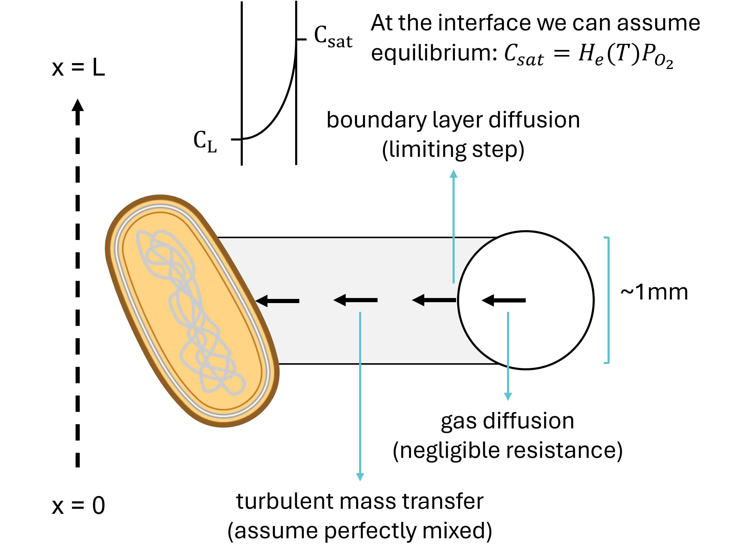
The basic mass tranfer equation at a height of x is therefore:
\(OTR = k_La(C_{sat} - C)_x\)
For tall vessels (>1 m tall), the oxygen concentration are significantly different at the top and bottom of the reactor. We can account for the O2 concentration gradient across the height by using the log-mean driving force:
\(OTR = k_La \frac{(C_{sat} - C)_{out} - (C_{sat} - C)_{in}}{ln\Big(\large \frac{(C_{sat} - C)_{out}}{(C_{sat} - C)_{in}} \Big)}\)
The \(k_La\) can be correlated to the superficail gas velocity, \(U_S\), and the agitator power per unit volume, \(P\), as follows:
\(k_La = AP^BU_S^C\)
Where A, B, and C are correlation coefficients dependent on the agitator system, broth type, and size dimensions. The detailed design of the agitator is not relevant at this stage of the analysis, but the correlation coefficients will be a function of the agitator design.
The saturated oxygen concentration can be estimated using Henry’s law:
\(C_{sat} = H \cdot P \cdot y\)
\(H = k_H \cdot exp(A \cdot (1/T - 1/T_{ref}))\)
Due to the liquid head, the pressure will vary across the tank as follows:
\(P = P_{atm} + g \rho (1 - x / L)\)
Where \(g\) is the acceleration due to gravity, \(\rho\) is the liquid density, and \(x\) is the height of the fluid.
When estimating the OTR, it is important to keep track of units of measure and make sure all are consistent with the coefficients/correlations being used. In the following code, we will use BioSTEAM functions for estimating the saturated oxygen concentration, the kLa, and ultimately estimate the air flow rate required to meet the oxygen uptake rate numerically.
Assumptions
Assume a dissolved oxygen concentration of 50% saturation. Note that the flow rate of air (or agitation power) required to achieve an oxygen uptake rate equal to the oxygen transfer rate will depend on the oxygen saturation.
Set the power consumed by the agitator to 0.2955 kW∙m3, a heuristic value common for industrial homogeneous reactions and comparable to estimates in Aspen plus. Note that is also possible to minimize power consumption by varying flow rate, but this would also lead to a greater capital cost for the compressor.
Assume the Van’t Riet’s non-viscous mass transfer correlation is applicable to estimate the overall mass transfer coefficient, kLa (lumped together with the specific interfacial area).
[13]:
from flexsolve import IQ_interpolation
g = bst.constants.g
theta_O2 = 0.5 # Dissolved oxygen concentration [% saturation]
kW_per_m3 = 0.2955 # Agitation power [kW / m3]
L = H * f # Length of filled vessel
air.P = g * broth.rho * L + 101325 # Inlet air pressure
vent.P = 101325 # Outlet air pressure

def objective(air_flow):
    air.set_flow([air_flow * 0.21, air_flow * 0.79], 'mol/s', ['O2', 'N2'])

    # React with oxygen
    vent.empty()
    broth.mix_from([feed, air], energy_balance=False) # Isothermal mixing
    fermentation(broth)

    # Perform vapor-liquid equilibrium
    aeration.vent_broth(vent, broth)

    # Estimate kLa
    V_reactive = V_reactor * f
    fraction_operating = tau_reaction / (tau_reaction + tau_cleanup + tau_loading)
    agitation_power = 1e3 * kW_per_m3 * V_reactive # Power input in W
    F = air.get_total_flow('m3/s') / N_reactors / fraction_operating
    r = 0.5 * D
    A = π * r * r
    superficial_gas_flow = U = F / A # m / s
    kLa = aeration.kLa_stirred_Riet(agitation_power, V_reactive, U) # 1 / s

    # Estimate OTR [mol / s]
    P_O2_air = air.get_property('P', 'bar') * air.imol['O2'] / air.F_mol
    P_O2_vent = vent.get_property('P', 'bar') * vent.imol['O2'] / vent.F_mol
    C_O2_sat_air = aeration.C_O2_L(T_operation, P_O2_air) # mol / kg
    C_O2_sat_vent = aeration.C_O2_L(T_operation, P_O2_vent) # mol / kg
    LMDF = aeration.log_mean_driving_force(C_O2_sat_vent, C_O2_sat_air, theta_O2 * C_O2_sat_vent, theta_O2 * C_O2_sat_air)
    OTR = kLa * LMDF * broth.rho * V_total * fraction_operating # mol / s

    # Return error in estimate
    return OUR - OTR

minimum_air_flow_rate = OUR / 0.21
maximum_air_flow_rate = 10 * minimum_air_flow_rate
IQ_interpolation(objective, minimum_air_flow_rate, maximum_air_flow_rate) # Solve air flow

# Show stream results
feed.show('cwt')
print()
air.show('cwt')
print()
vent.show('cwt')
print()
broth.show('cwt')
print()
print('Titer:', f'{broth.imass['MicrobialOil'] / broth.F_vol:.3g}', '[g/L]')
Stream: feed
phase: 'l', T: 305.15 K, P: 101325 Pa
flow (%): Glucose  14.5
          Water    85.5
          -------  1.03e+05 kg/hr

Stream: air
phase: 'g', T: 305.15 K, P: 256924 Pa
flow (%): O2  23.3
          N2  76.7
          --  1.92e+04 kg/hr

Stream: vent
phase: 'g', T: 305.15 K, P: 101325 Pa
flow (%): Water  2.7
          CO2    25.2
          O2     12.2
          N2     59.9
          -----  2.45e+04 kg/hr

Stream: broth
phase: 'l', T: 305.15 K, P: 101325 Pa
flow (%): Water         92.9
          CO2           0.0216
          O2            0.000449
          N2            0.00108
          MicrobialOil  2.76
          Yeast         4.34
          ------------  9.79e+04 kg/hr

Titer: 27.5 [g/L]
Note how the titer increased by 0.1 g/L (0.4%) after adjusting the air flow rate. This is because the off-gas is at 100% humidity and increasing the air flow rate carries away a small fraction of the water. To strictly meet the titer specification (at a lower margin of error), we can repeatedly solve for the dilution water and air flow rate until we converge. In this tutorial, we assume that a 0.4% error is good enough.
22.3.4. Energy balance & heat transfer#
We can design the heat transfer configuration as a jacketed vessel. The same equations as the anaerobic bioreactor apply to solve for the cooling duty and the flow rate of the chilled water required to achieve the heat transfer requirement.
Note that estimating the overall heat transfer coefficient can be challenging due to its dependence on detailed design of the bioreactor (e.g., agitation) and mixture properties (e.g., density, conductivity). As a preliminary estimate, we will assume that the temperature of the outlet utility is simply the maximum allowable temperature for smooth regeneration (chilled water cannot come back too hot to the cooler). Because the cost of chilled water usage is estimated based on the total heat transfered (not on the actual flow rate), this assumption does not impact our economic analysis.
[14]:
# Enthalpy change (including heats of formation)
cooling_duty = (product.Hf + product.H) - (feed.Hf + feed.H)

# Additional assumptions/specifications
T_utility_out = 27.22 + 273.15
T_utility_in = 7.22 + 273.15

# Solve for utility requirements
chilled_water_in = bst.Stream(Water=1, T=T_utility_in)
chilled_water_out = bst.Stream(Water=1, T=T_utility_out)
F_utility = cooling_duty / (chilled_water_in.h - chilled_water_out.h)

print('Cooling duty:', f'{cooling_duty:.3g}', 'kJ/hr')
print('Chilled water flow rate:',  f'{F_utility:.3g}', 'kmol/hr')
Cooling duty: -3.94e+07 kJ/hr
Chilled water flow rate: 2.61e+04 kmol/hr
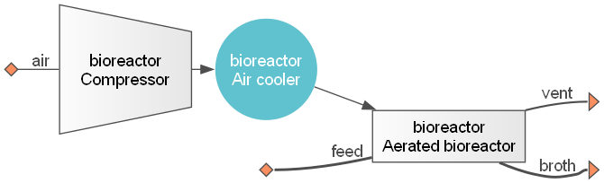
22.3.5. Aerated bioreactor model#
Let’s use BioSTEAM’s AeratedBioreactor model to model the production of microbial oil by fermentation:
[15]:
bioreactor = bst.AeratedBioreactor(
    ins=feed,
    outs=('vent', 'broth'),
    reactions=fermentation,
    T=T_operation,
    V_wf=f,
    V_max=V_max,
    tau=tau_reaction,
    tau_0=tau_cleanup,
    loading_time=tau_loading,
    length_to_diameter=R,
    method='Riet', # Name of method; Alternatively, 'Dewes' for bubble columns
    design='Stirred tank',  # Reactor type; Alternatively, 'Bubble column'
    heat_exchanger_configuration='jacketed',
    kW_per_m3=kW_per_m3,
    # Option to adjust both compressor and agitation power
    # to minimize the sum of both, yet still meet mass tranfer requirement
    optimize_power=False,
)
bioreactor.simulate()
bioreactor.diagram(format='png')
bioreactor.show('cwt')
print()
broth = bioreactor.outs[1]
print('Titer:', f'{broth.imass['MicrobialOil'] / broth.F_vol:.3g}', '[g/L]')
print()
bioreactor.results()
AeratedBioreactor: bioreactor
ins...
[0] feed
    phase: 'l', T: 305.15 K, P: 101325 Pa
    flow (%): Glucose  14.5
              Water    85.5
              -------  1.03e+05 kg/hr
[1] air
    phase: 'g', T: 305.15 K, P: 101325 Pa
    flow (%): O2  23.3
              N2  76.7
              --  2.04e+04 kg/hr
outs...
[0] vent
    phase: 'g', T: 305.15 K, P: 101325 Pa
    flow (%): Water  2.72
              CO2    23.9
              O2     12.7
              N2     60.6
              -----  2.59e+04 kg/hr
[1] broth
    phase: 'l', T: 305.15 K, P: 101325 Pa
    flow (%): Water         92.9
              CO2           0.0204
              O2            0.000466
              N2            0.00109
              MicrobialOil  2.76
              Yeast         4.34
              ------------  9.78e+04 kg/hr

Titer: 27.5 [g/L]
[15]:
| Aerated bioreactor | Units | bioreactor | |
|---|---|---|---|
| Electricity | Power | kW | 3.57e+03 |
| Cost | USD/hr | 279 | |
| Chilled water | Duty | kJ/hr | -4.2e+07 |
| Flow | kmol/hr | 2.81e+04 | |
| Cost | USD/hr | 210 | |
| Design | Reactor volume | m3 | 482 |
| Batch time | hr | 92 | |
| Loading time | hr | 1 | |
| Number of reactors | 21 | ||
| Residence time | hr | 88 | |
| Vessel type | Vertical | ||
| Length | ft | 58 | |
| Diameter | ft | 19.3 | |
| Weight | lb | 1.38e+05 | |
| Wall thickness | in | 0.401 | |
| Jacketed diameter | ft | 19.5 | |
| Vessel material | Stainless steel 316 | ||
| Purchase cost | Vertical pressure vessel (jacketed) (x21) | USD | 5.73e+06 |
| Platform and ladders (x21) | USD | 1.36e+06 | |
| Compressor - Compressor(s) (x21) | USD | 6.44e+05 | |
| Air cooler - Floating head (x21) | USD | 2.11e+04 | |
| Agitator - Agitator (x21) | USD | 1.62e+06 | |
| Total purchase cost | USD | 9.38e+06 | |
| Installed equipment cost | USD | 2.83e+07 | |
| Utility cost | USD/hr | 490 |
Note how our calculations match BioSTEAM’s results on bioreactor size and stream flow rates. The required cooling duty and chilled water flow rate are higher in the unit operation because the air is also cooled after the compressor.
[16]:
bioreactor.compressor.show('cwt')
print()
bioreactor.compressor.results()
IsentropicCompressor: compressor
ins...
[0] air
    phase: 'g', T: 305.15 K, P: 101325 Pa
    flow (%): O2  23.3
              N2  76.7
              --  2.04e+04 kg/hr
outs...
[0] to  HXutility-air_cooler
    phase: 'g', T: 427.32 K, P: 284671 Pa
    flow (%): O2  23.3
              N2  76.7
              --  2.04e+04 kg/hr
[16]:
| Isentropic compressor | Units | compressor | |
|---|---|---|---|
| Electricity | Power | kW | 882 |
| Cost | USD/hr | 69 | |
| Design | Ideal power | kW | 600 |
| Ideal duty | kJ/hr | 0 | |
| Type | Screw | ||
| Compressors in parallel | 1 | ||
| Driver | Electric motor | ||
| Driver efficiency | 0.8 | ||
| Purchase cost | Compressor(s) | USD | 6.44e+05 |
| Total purchase cost | USD | 6.44e+05 | |
| Installed equipment cost | USD | 1.38e+06 | |
| Utility cost | USD/hr | 69 |
22.4. Gas-fed acetic acid bioreactor#
Microbial carbon utilization technologies may help maximize product yields, displace environmental impacts, and reduce fossil fuel consumption. Among such pathways, there is a range of alternative flue gas sources and possible fermentation products. Using flue gas from a coal-powered steel mill, a pilot-scale gas-fed fermentation process reported negative carbon intensities (−1.78 kgCO2e·kg-1 acetone and −1.17 kgCO2e·kg-1 isopropanol), which is possible because carbon is fixed into small organic molecules.
Modeling a gas-fed fermentation process leverages all the same equations and design algorithms as an aerated bioreactor with the added complexity that the main substrates are now in gas feeds. The detailed example calculations will be added in the future. For now, let’s move directly to using BioSTEAM’s GaseFedBioreactor to model the production of acetic acid by fermentating flue gas and acetic acid:
[27]:
import biosteam as bst
bst.settings.set_thermo(['H2', 'CO2', 'CO', 'N2', 'O2', 'H2O', 'AceticAcid'])

# Feeds
media = bst.Stream(ID='media', H2O=20e3, units='kg/hr')
H2 = bst.Stream(ID='H2', H2=100, units='kg/hr', phase='g')
fluegas = bst.Stream(CO=23, CO2=23, H2=4.5, N2=49.5, units='m3/hr', phase='g')
H2.F_mass = 5e3
fluegas.F_mass = 8e3

# Model acetic acid production from H2 and CO2
rxn = bst.SeriesReaction([
    bst.Reaction(
        'CO + H2O -> CO2 + H2',
        reactant='CO', correct_atomic_balance=True, X=1
    ),
    bst.Reaction(
        'H2 + CO2 -> AceticAcid + H2O',
        reactant='CO2', correct_atomic_balance=True, X=1
    ),
])
bioreactor = bst.GasFedBioreactor(
    ins=[media, H2, fluegas],
    outs=('vent', 'product'),
    tau=68, V_max=500,
    length_to_diameter=6,
    reactions=rxn,
    gas_substrates=('H2', 'CO', 'CO2'),
    design='Bubble column',
    kW_per_m3=0,
    batch=False,
    T=305.15
)
bioreactor.simulate()
bioreactor.show('cwt')
print()
bioreactor.results()
GasFedBioreactor: bioreactor
ins...
[0] media
    phase: 'l', T: 298.15 K, P: 101325 Pa
    flow: 2e+04 kg/hr H2O
[1] H2
    phase: 'g', T: 298.15 K, P: 101325 Pa
    flow: 5e+03 kg/hr H2
[2] fluegas
    phase: 'g', T: 298.15 K, P: 101325 Pa
    flow (%): H2   0.296
              CO2  33.3
              CO   21.1
              N2   45.4
              ---  8e+03 kg/hr
outs...
[0] vent
    phase: 'g', T: 305.15 K, P: 101325 Pa
    flow (%): H2          0.51
              CO2         98
              H2O         1.36
              AceticAcid  0.12
              ----------  1.31e+03 kg/hr
[1] product
    phase: 'l', T: 305.15 K, P: 101325 Pa
    flow (%): H2          2.42e-05
              CO2         0.106
              H2O         95.7
              AceticAcid  4.17
              ----------  2.14e+04 kg/hr
[27]:
| Gas fed bioreactor | Units | bioreactor | |
|---|---|---|---|
| Electricity | Power | kW | 3.93e+03 |
| Cost | USD/hr | 308 | |
| Chilled water | Duty | kJ/hr | -1.07e+07 |
| Flow | kmol/hr | 7.12e+03 | |
| Cost | USD/hr | 53.7 | |
| Low pressure steam | Duty | kJ/hr | 4e+06 |
| Flow | kmol/hr | 103 | |
| Cost | USD/hr | 24.6 | |
| Design | Reactor volume | m3 | 426 |
| Number of reactors | 4 | ||
| Residence time | hr | 68 | |
| Vessel type | Vertical | ||
| Length | ft | 88.4 | |
| Diameter | ft | 14.7 | |
| Weight | lb | 9.14e+04 | |
| Wall thickness | in | 0.493 | |
| Vessel material | Stainless steel 316 | ||
| Purchase cost | Vertical pressure vessel (x4) | USD | 1.71e+06 |
| Platform and ladders (x4) | USD | 2.85e+05 | |
| Compressors[0] - Compressor(s) (x4) | USD | 2.14e+06 | |
| Compressors[1] - Compressor(s) (x4) | USD | 3.43e+05 | |
| Gas coolers[0] - Floating head (x4) | USD | 2.86e+04 | |
| Gas coolers[1] - Double pipe (x4) | USD | 5.18e+03 | |
| Heat exchanger - Double pipe (x4) | USD | 1.9e+04 | |
| Recirculation pump - Pump (x4) | USD | 1.83e+04 | |
| Recirculation pump - Motor (x4) | USD | 1.8e+03 | |
| Total purchase cost | USD | 4.55e+06 | |
| Installed equipment cost | USD | 1.01e+07 | |
| Utility cost | USD/hr | 386 |
The optimal design of the gas-fed fermentation bioreactors (e.g., height, operating pressure, agitation, H2 and flue gas feed ratios) and the downstream separation configuration will be unique for each fermentation performance scenario (i.e., titer, rate, yield) and can significantly impact costs and performance.