29. Solvent-targeted plastic dissolution and precipitation (STRAP)#
29.1. Basics#
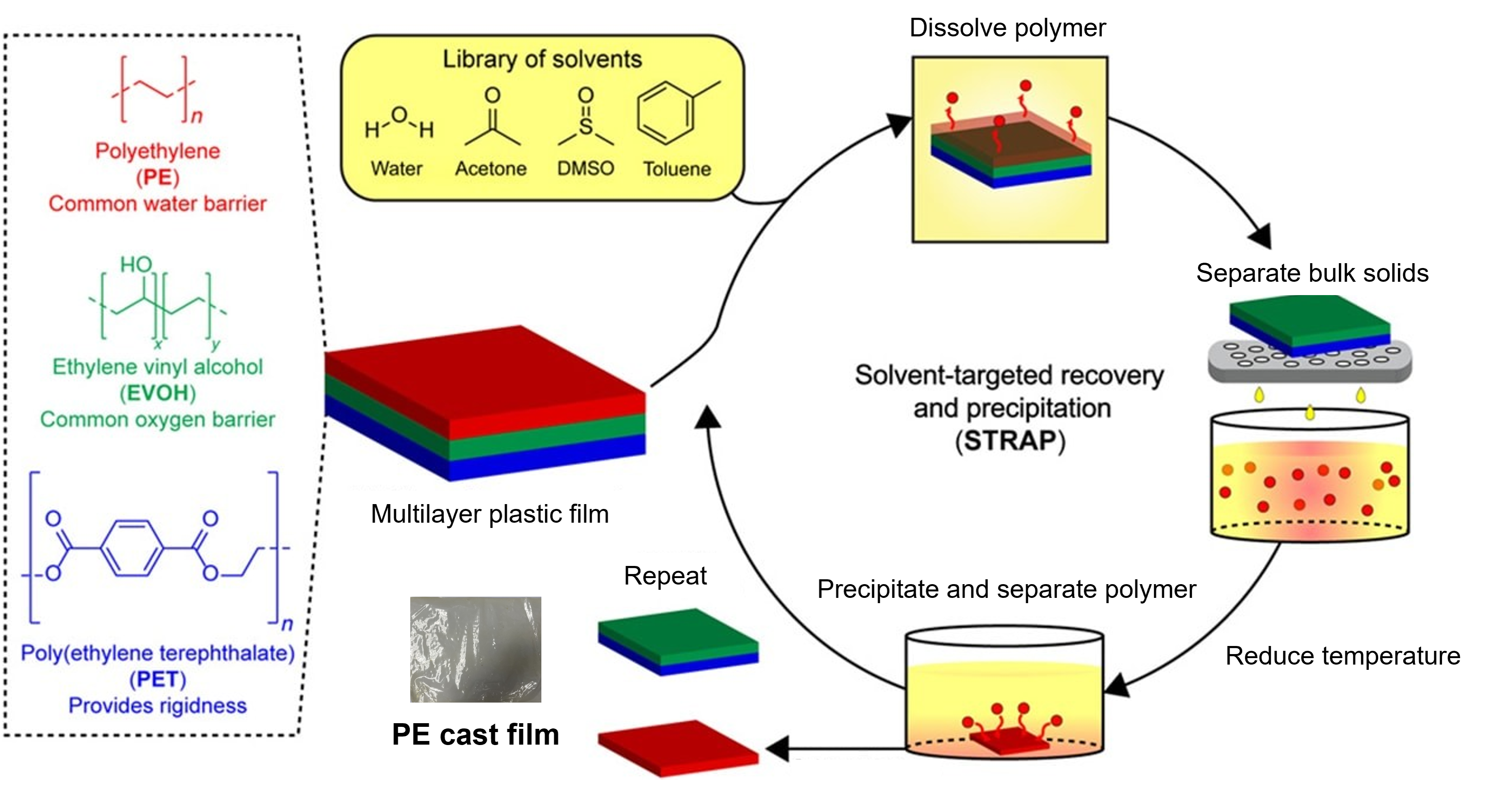
It is often said that we live in the plastics age. Plastics are consumed across all sectors (clothing, medicine, construction, food packaging) as plastics are versatile, low cost, and easy to manufacture. However, the final disposal of plastics is a global concern. Multilayer films are among the most challenging plastic wastes to recycle, but the STRAP technology can recover the individual plastic components, known as resins. STRAP “washes” multilayered films several times with solvents to separate each resin at a time. These resins can then be reused to make more of the product from which they originated, or they can be used to manufacture products with higher value or quality (known as upcycling).
29.2. Process configuration#
We will be looking at a STRAP process model for the separation of post-industrial multilayered plastic film composed of PE, EvOH, and PET. Many uncertainties exist for this emerging technology, such as the relative amount PE in the film and the amount of solvent required to dissolve it.
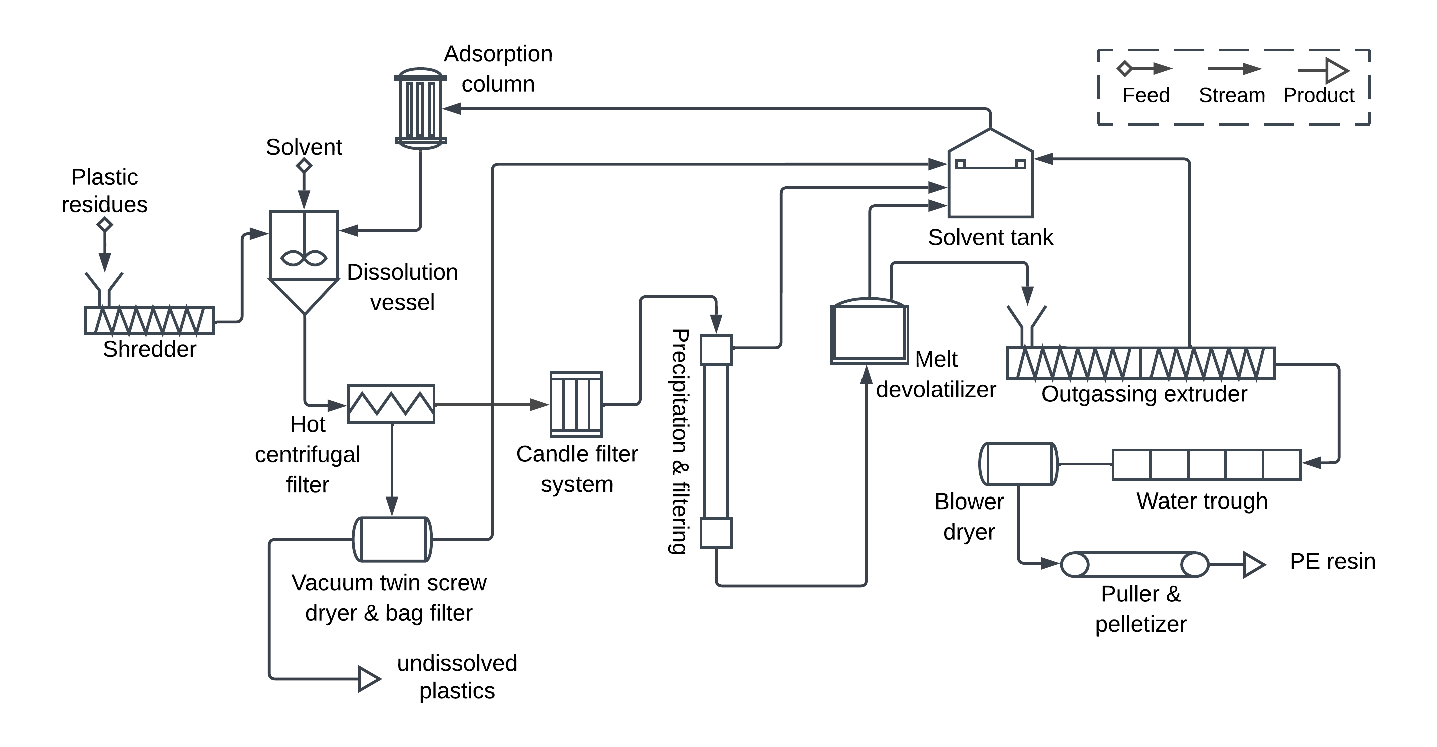
A preliminary STRAP process model was developed in BioSTEAM with roughly the flowsheet configuration shown in the figure. Note that the flowsheet shows only one cycle of a dissolution and precipitation step, but two cycles are needed to separate all components in the figure (PE, EvOH, PET).
In this tutorial, we will push and pull the STRAP process models coded in BioSTEAM to understand the potential economic and environmental impact of the following design configurations:
Single layer (PE) separation with burning of remaining plastic for heat and power.
Multilayer separation of PE and EVOH in two-step process with selling the remaining coproduct.
Techno-economic and life cycle assessment of these conceptual scenarios will help us analyse the feasibility of the STRAP process for recycling multilayer plastics and the trade-offs in potential design decisions. We will also explore the sensitivity of each configuration to key assumptions on feedstock composition and technological performance.
29.3. Single layer (PE) separation#
Before loading the process model, let’s have a look at predefined scenarios within the BaselineSTRAPProcess class (the main interface to the process model):
[1]:
import biosteam as bst
from cuwp import strap
bst.nbtutorial() # enable interactive diagrams
scenarios = strap.BaselineSTRAPProcess.get_scenarios()
metadata = True
for i in scenarios[:3]:
    i.show(metadata)
    metadata = False
Scenario(
    # Solvent used to separate the target plastic
    solvent='THF',
    # The polymer layer being dissolved
    target_plastic='PC',
    # Fraction in feedstock [%]
    target_plastic_percent=65,
    # Feedstock flow rate [MT-plastic/yr]
    processing_capacity=250,
    # Whether the MSP will include all products
    sell_leftover_plastic=False,
    # Produce heat and power from leftover plastic
    burn_leftover_plastic=False,
    # On-site heat and power generation
    facilities=False,
    # Use 'drop' for % temperature drop to solvent melting point. Use 'constant' to set in Kelvin.
    precipitation_temperature_format='constant',
    # Must be either 'solvent mixing' or 'integrated heat transfer'.
    precipitation_configuration='integrated heat transfer',
    # On-site electricity generation
    turbogenerator=True,
    # Percent inks and solubles
    percent_inks=None,
    # On-site cooling tower
    cooling_tower=True,
)
Scenario(
    solvent='Toluene',
    target_plastic='PE',
    target_plastic_percent=50,
    processing_capacity=5e+03,
    sell_leftover_plastic=False,
    burn_leftover_plastic=True,
    facilities=True,
    precipitation_temperature_format='constant',
    precipitation_configuration='integrated heat transfer',
    turbogenerator=True,
    percent_inks=None,
    cooling_tower=True,
)
Scenario(
    solvent=('Toluene', 'DMSOWater'),
    target_plastic=('PE', 'EVOH'),
    target_plastic_percent=(50, 3.22),
    processing_capacity=5e+03,
    sell_leftover_plastic=False,
    burn_leftover_plastic=True,
    facilities=True,
    precipitation_temperature_format='constant',
    precipitation_configuration='integrated heat transfer',
    turbogenerator=True,
    percent_inks=None,
    cooling_tower=True,
)
In each scenario, there can be one or more targeted plastics. The rest of the plastic is considered to be a generic “bulk plastic” with the same properties (e.g., molecular weight, formula, density, heat capacity) as PET. The facilities argument defines whether to include the production of utilities (e.g., cooling water, steam, power) on-site. It is recomended to include facilities when the processing capacity is high.
Let’s load the process model using the scenario where the target plastic is ‘PE’, the solvent is ‘Toluene’, and the leftover plastic is sent to on-site heat and power generation:
[2]:
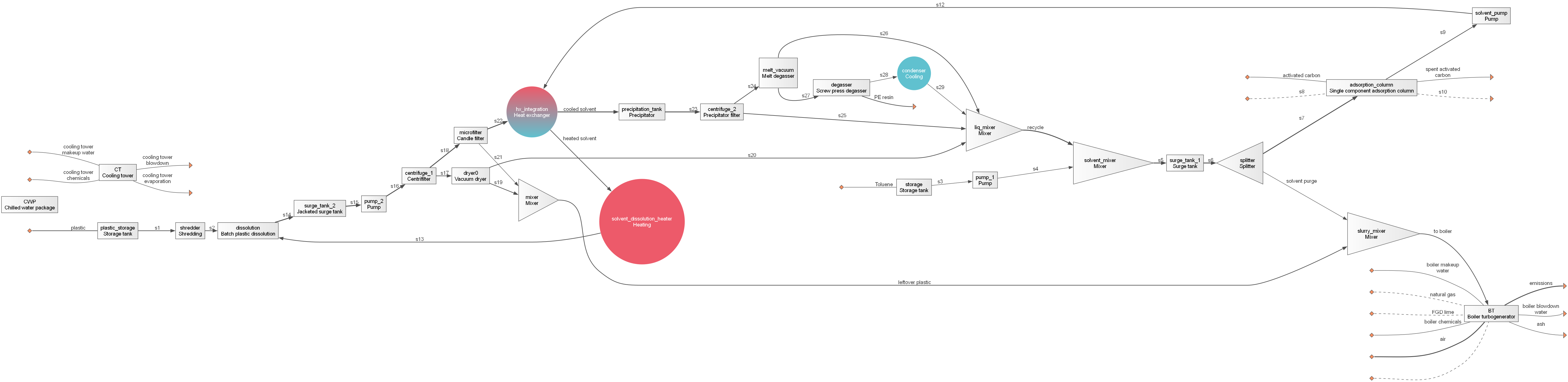
process = strap.BaselineSTRAPProcess(scenario='PE/Toluene')
process.system.diagram(format='png') # Note how the leftover plastic is sent to heat and power generation.
process.show()
BaselineSTRAPProcess(
    # Solvent used to separate the target plastic
    solvent='Toluene',
    # The polymer layer being dissolved
    target_plastic='PE',
    # Fraction in feedstock [%]
    target_plastic_percent=50,
    # Feedstock flow rate [MT-plastic/yr]
    processing_capacity=5e+03,
    # Whether the MSP will include all products
    sell_leftover_plastic=False,
    # Produce heat and power from leftover plastic
    burn_leftover_plastic=True,
    # On-site heat and power generation
    facilities=True,
    # Use 'drop' for % temperature drop to solvent melting point. Use 'constant' to set in Kelvin.
    precipitation_temperature_format='constant',
    # Must be either 'solvent mixing' or 'integrated heat transfer'.
    precipitation_configuration='integrated heat transfer',
    # On-site electricity generation
    turbogenerator=True,
    # Percent inks and solubles
    percent_inks=None,
    # On-site cooling tower
    cooling_tower=True,
)
In addition to the scenario specifications, this process model has number of other assumtions. Let’s have a look as the baseline assumptions and results:
[3]:
assumptions, results = process.baseline()
assumptions
| 0 | ||
|---|---|---|
| Natural gas | Price [USD/m3] | 0.167 |
| Feedstock | Processing capacity [MT/yr] | 5e+03 |
| Price [USD/kg] | 0.01 | |
| feedstock | Distance [km] | 500 |
| Cashflow analysis | IRR [%] | 0.1 |
| target polymer | Mass fraction | 0.5 |
| centrifuged plastic | Solvent content [%] | 50 |
| Solvent | Price [USD/kg] | 2.17 |
| solvent | Solvent loss [%] | 0.1 |
| dissolution | Solvent capacity [wt %] | 3 |
| Temperature [K] | 368 | |
| precipitation | Temperature [K] | 308 |
[4]:
results
| 0 | ||
|---|---|---|
| - | GWP [kg*CO2e/kg] | 1.57 |
| FFC [MJ/kg] | 0.948 | |
| WU [m3/kg] | -0.679 | |
| MSP [USD/kg] | 2.81 |
Every unit operation and stream are available as attributes in the model:
[7]:
process.dissolution.show('cwt')
BatchPlasticDissolution: dissolution
ins...
[0] s2  from  Shredding-shredder
    phase: 'l', T: 298.15 K, P: 101325 Pa
    composition (%): PE           50
                     BulkPlastic  50
                     Solubles     0.0001
                     -----------  595 kg/hr
[1] s13  from  HXutility-solvent_dissolution_heater
    phase: 'l', T: 368.15 K, P: 1.01325e+06 Pa
    composition (%): Toluene   100
                     Minerals  1.29e-05
                     --------  9.9e+03 kg/hr
outs...
[0] s14  to  StorageTank-surge_tank_2
    phase: 'l', T: 365.18 K, P: 101325 Pa
    composition (%): Toluene      94.3
                     PEoligomer   2.83
                     BulkPlastic  2.83
                     Minerals     1.22e-05
                     Solubles     5.66e-06
                     -----------  1.05e+04 kg/hr
[8]:
process.dissolution.results(basis='SI')
[8]:
| Batch plastic dissolution | Units | dissolution | |
|---|---|---|---|
| Electricity | Power | kW | 6.39 |
| Cost | USD/hr | 0.447 | |
| Design | Reactor volume | m³ | 8.11 |
| Residence time | hr | 0.5 | |
| Vessel type | Vertical | ||
| Length | m | 4.53 | |
| Diameter | m | 1.51 | |
| Weight | kg | 1.61e+03 | |
| Wall thickness | m | 0.00794 | |
| Vessel material | Stainless steel 304 | ||
| Purchase cost | Vertical pressure vessel | USD | 6.36e+04 |
| Platform and ladders | USD | 1.3e+04 | |
| Agitator - Agitator | USD | 2.01e+04 | |
| Total purchase cost | USD | 9.67e+04 | |
| Utility cost | USD/hr | 0.447 |
More details for techno-economic analysis (TEA) and life cycle asssessment (LCA) :
[9]:
process.tea.get_cashflow_table()
[9]:
| Depreciable capital [MM$] | Fixed capital investment [MM$] | Working capital [MM$] | Depreciation [MM$] | Loan [MM$] | ... | Net earnings [MM$] | Cash flow [MM$] | Discount factor | Net present value (NPV) [MM$] | Cumulative NPV [MM$] | |
|---|---|---|---|---|---|---|---|---|---|---|---|
| 2022 | 3.03 | 3.19 | 0 | 0 | 0 | ... | 0 | -3.19 | 1.21 | -3.87 | -3.87 |
| 2023 | 22.7 | 24 | 0 | 0 | 0 | ... | 0 | -24 | 1.1 | -26.4 | -30.2 |
| 2024 | 12.1 | 12.8 | 2 | 0 | 0 | ... | 0 | -14.8 | 1 | -14.8 | -45 |
| 2025 | 0 | 0 | 0 | 4.53 | 0 | ... | -0.847 | 3.68 | 0.909 | 3.35 | -41.7 |
| 2026 | 0 | 0 | 0 | 7.83 | 0 | ... | -3.4 | 4.43 | 0.826 | 3.66 | -38 |
| 2027 | 0 | 0 | 0 | 5.72 | 0 | ... | -1.28 | 4.43 | 0.751 | 3.33 | -34.7 |
| 2028 | 0 | 0 | 0 | 4.2 | 0 | ... | 0.232 | 4.43 | 0.683 | 3.03 | -31.6 |
| 2029 | 0 | 0 | 0 | 3.11 | 0 | ... | 1.32 | 4.43 | 0.621 | 2.75 | -28.9 |
| 2030 | 0 | 0 | 0 | 3.07 | 0 | ... | 1.36 | 4.43 | 0.564 | 2.5 | -26.4 |
| 2031 | 0 | 0 | 0 | 3.04 | 0 | ... | 1.39 | 4.43 | 0.513 | 2.27 | -24.1 |
| 2032 | 0 | 0 | 0 | 1.69 | 0 | ... | 2.42 | 4.11 | 0.467 | 1.92 | -22.2 |
| 2033 | 0 | 0 | 0 | 0.371 | 0 | ... | 3.21 | 3.58 | 0.424 | 1.52 | -20.7 |
| 2034 | 0 | 0 | 0 | 0.371 | 0 | ... | 3.21 | 3.58 | 0.386 | 1.38 | -19.3 |
| 2035 | 0 | 1.06e-06 | 0 | 0.371 | 0 | ... | 3.21 | 3.58 | 0.35 | 1.25 | -18 |
| 2036 | 0 | 0 | 0 | 0.371 | 0 | ... | 3.21 | 3.58 | 0.319 | 1.14 | -16.9 |
| 2037 | 0 | 0 | 0 | 0.371 | 0 | ... | 3.21 | 3.58 | 0.29 | 1.04 | -15.9 |
| 2038 | 0 | 0 | 0 | 0.371 | 0 | ... | 3.21 | 3.58 | 0.263 | 0.943 | -14.9 |
| 2039 | 0 | 0 | 0 | 0.371 | 0 | ... | 3.21 | 3.58 | 0.239 | 0.857 | -14.1 |
| 2040 | 0 | 1.06e-06 | 0 | 0.371 | 0 | ... | 3.21 | 3.58 | 0.218 | 0.779 | -13.3 |
| 2041 | 0 | 0 | 0 | 0.371 | 0 | ... | 3.21 | 3.58 | 0.198 | 0.708 | -12.6 |
| 2042 | 0 | 0 | 0 | 0.371 | 0 | ... | 3.21 | 3.58 | 0.18 | 0.644 | -11.9 |
| 2043 | 0 | 0 | 0 | 0.371 | 0 | ... | 3.21 | 3.58 | 0.164 | 0.585 | -11.3 |
| 2044 | 0 | 0 | 0 | 0.371 | 0 | ... | 3.21 | 3.58 | 0.149 | 0.532 | -10.8 |
| 2045 | 0 | 1.06e-06 | 0 | 0.186 | 0 | ... | 3.35 | 3.54 | 0.135 | 0.478 | -10.3 |
| 2046 | 0 | 0 | 0 | 0 | 0 | ... | 3.5 | 3.5 | 0.123 | 0.43 | -9.9 |
| 2047 | 0 | 0 | 0 | 0 | 0 | ... | 3.5 | 3.5 | 0.112 | 0.391 | -9.51 |
| 2048 | 0 | 0 | 0 | 0 | 0 | ... | 3.5 | 3.5 | 0.102 | 0.355 | -9.15 |
| 2049 | 0 | 0 | 0 | 0 | 0 | ... | 3.5 | 3.5 | 0.0923 | 0.323 | -8.83 |
| 2050 | 0 | 1.06e-06 | 0 | 0 | 0 | ... | 3.5 | 3.5 | 0.0839 | 0.294 | -8.53 |
| 2051 | 0 | 0 | 0 | 0 | 0 | ... | 3.5 | 3.5 | 0.0763 | 0.267 | -8.27 |
| 2052 | 0 | 0 | 0 | 0 | 0 | ... | 3.5 | 3.5 | 0.0693 | 0.243 | -8.02 |
| 2053 | 0 | 0 | 0 | 0 | 0 | ... | 3.5 | 3.5 | 0.063 | 0.221 | -7.8 |
| 2054 | 0 | 0 | -2 | 0 | 0 | ... | 3.5 | 5.5 | 0.0573 | 0.315 | -7.49 |
33 rows × 19 columns
[10]:
products = [process.PE_resin]
bst.report.lca_inventory_table(
    [process.system], 'GWP', products
) # Surplus electricity is produced when leftover plastic is burned for heat and power
[10]:
| Inventory [kg/yr] | ||
|---|---|---|
| Inputs | Toluene | 4.17e+04 |
| Plastic | 5e+06 | |
| Cooling water | 8.47e+07 | |
| Outputs | PE resin | 2.43e+06 |
| Electricity [kWhr/yr] | 6.9e+06 | |
| Direct non-biogenic emissions | 6.23e+06 |
The process model streamlines simulation, TEA, and LCA through parameters you can modify and system-wide metrics you can compute:
[11]:
process.model.show()
Model:
parameters: Natural gas - Price [USD/m3]
            Feedstock - Processing capacity [MT/yr]
            Feedstock - Price [USD/kg]
            Feedstock - Distance [km]
            Cashflow analysis - IRR [%]
            Target polymer - Mass fraction
            Centrifuged plastic - Solvent content [%]
            Solvent - Price [USD/kg]
            Solvent - Solvent loss [%]
            Dissolution - Solvent capacity [wt %]
            Dissolution - Temperature [K]
            Precipitation - Temperature [K]
indicators: GWP [kg*CO2e/kg]
            FFC [MJ/kg]
            WU [m3/kg]
            MSP [USD/kg]
[12]:
process.MSP(), process.GWP() # Get minimum selling price and carbon intensity
[12]:
(2.8093356553821254, 1.5677679774244218)
[13]:
process.set_polymer_mass_fraction(0.4) # Set PE fraction
process.system.simulate() # Rerun system
process.MSP(), process.GWP() # Get minimum selling price and carbon intensity
[13]:
(3.370088060045807, 2.0450682109041343)
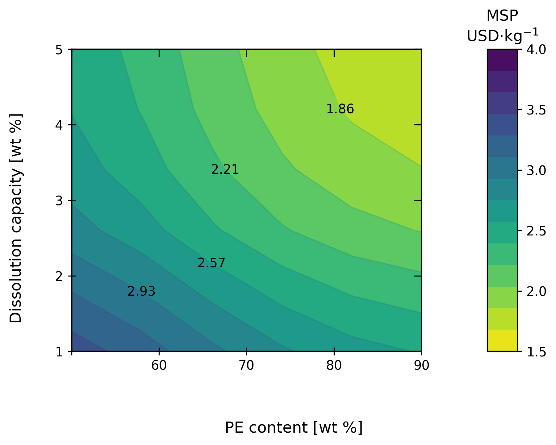
29.4. Sensitivity analysis#
Now that we understand the model, we can evaluate it across potential compositions and dissolution capacities to understand the potential impact of these assumptions.
[14]:
import numpy as np
from matplotlib import pyplot as plt

def MSP_at_PE_mass_fraction_and_dissolution_capacity(mass_fraction, dissolution_capacity, process):
    process.set_polymer_mass_fraction(mass_fraction)
    process.set_dissolution_capacity(dissolution_capacity)
    process.system.simulate()
    return process.MSP()

xlim = np.array([0.5, 0.9])
ylim = np.array([1, 5])
X, Y, Z = bst.plots.generate_contour_data(
    MSP_at_PE_mass_fraction_and_dissolution_capacity,
    xlim=xlim, ylim=ylim, args=(process,),
    n=6,
)

# Plot contours
xlabel = "PE content [wt %]"
ylabel = 'Dissolution capacity [wt %]'
xticks = [50, 60, 70, 80, 90]
yticks = [1, 2, 3, 4, 5]
metric_bar = bst.plots.MetricBar(
    'MSP', 'USD$\cdot$kg$^{-1}$', plt.cm.get_cmap('viridis_r'),
    [1.5, 2, 2.5, 3, 3.5, 4], 15, 2
)
fig, axes, CSs, CB, other_axes = bst.plots.plot_contour_single_metric(
    100 * X, Y, Z[:, :, None, None], xlabel, ylabel, xticks, yticks, metric_bar,
    fillcolor=None, styleaxiskw=dict(xtick0=False), label=True,
)
29.5. Multilayer (PE, EVOH) separation#
Let’s move on to the separation of PE and EVOH with selling the remaining coproduct. This scenario is not an option in the process model, so we will need to provide the input assumption:
[15]:
assumptions, results = process.baseline()
assumptions
| 0 | ||
|---|---|---|
| Natural gas | Price [USD/m3] | 0.167 |
| Feedstock | Processing capacity [MT/yr] | 5e+03 |
| Price [USD/kg] | 0.01 | |
| feedstock | Distance [km] | 500 |
| Cashflow analysis | IRR [%] | 0.1 |
| target polymer | Mass fraction | 0.5 |
| centrifuged plastic | Solvent content [%] | 50 |
| Solvent | Price [USD/kg] | 2.17 |
| solvent | Solvent loss [%] | 0.1 |
| dissolution | Solvent capacity [wt %] | 3 |
| Temperature [K] | 368 | |
| precipitation | Temperature [K] | 308 |
[16]:
import biosteam as bst
from cuwp import strap
bst.nbtutorial()
process = strap.BaselineSTRAPProcess(
    target_plastic=('PE', 'EVOH'),
    target_plastic_percent=(50, 3.22), # %
    solvent=('Toluene', 'DMSOWater'),
    processing_capacity=5e+03, # MT/yr
    sell_leftover_plastic=True,
    burn_leftover_plastic=False,
    facilities=True,
)
process.system.diagram(format='png') # Note how the leftover plastic is now a product.
[17]:
# Includes the following results:
# global warming potential
# fossil fuel consumption
# water usage
# minimum selling price
results
| 0 | ||
|---|---|---|
| - | GWP [kg*CO2e/kg] | 1.57 |
| FFC [MJ/kg] | 0.948 | |
| WU [m3/kg] | -0.679 | |
| MSP [USD/kg] | 2.81 |
Under baseline assumptions, selling all layers of the film is more economically viable and has a lower environmental impact. Let’s see how the sensitivity analysis changes:
[18]:
import numpy as np
from matplotlib import pyplot as plt

def MSP_at_PE_mass_fraction_and_dissolution_capacity(mass_fraction, dissolution_capacity, process):
    process.set_polymer_mass_fraction(mass_fraction)
    process.set_PE_dissolution_capacity(dissolution_capacity)
    process.system.simulate()
    return process.MSP()

xlim = np.array([0.5, 0.9])
ylim = np.array([1, 5])
X, Y, Z = bst.plots.generate_contour_data(
    MSP_at_PE_mass_fraction_and_dissolution_capacity,
    xlim=xlim, ylim=ylim, args=(process,),
    n=6,
)

# Plot contours
xlabel = "PE content [wt %]"
ylabel = 'Dissolution capacity [wt %]'
xticks = [50, 60, 70, 80, 90]
yticks = [1, 2, 3, 4, 5]
metric_bar = bst.plots.MetricBar(
    'MSP', 'USD$\cdot$kg$^{-1}$', plt.cm.get_cmap('viridis_r'),
    [1.4, 1.8, 2.2, 2.6], 15, 2
)
fig, axes, CSs, CB, other_axes = bst.plots.plot_contour_single_metric(
    100 * X, Y, Z[:, :, None, None], xlabel, ylabel, xticks, yticks, metric_bar,
    fillcolor=None, styleaxiskw=dict(xtick0=False), label=True,
)
From the contour plot, we can see that the process economics favors a lower fraction of PE given how the leftover plastic is being sold as well.
29.6. Expanding the model to other polymer/solvent pairs.#
It is possible to expand the process model to any plastic/solvent pairs without limit on the number of layer separation steps. In the next example, we define a new plastic film and solvent pair, PEPP (PE and PP) and Xylene.
[19]:
import biosteam as bst
from cuwp import strap
bst.nbtutorial()
process = strap.BaselineSTRAPProcess(
    target_plastic='PEPP',
    target_plastic_percent=50, # %
    solvent='Xylene',
    processing_capacity=5e+03, # MT/yr
    sell_leftover_plastic=True,
    burn_leftover_plastic=False,
    facilities=False,
)
process.system.diagram(format='png') # Note how the leftover plastic is now a product.
[20]:
process.MSP()
[20]:
1.0593704734561622
Many assumptions were made in the creation of this scenario (e.g., dissolution capacity, dissolution temperature, precipitation temperature). For more detailed control over assumptions, use the strap.define_dissolution and strap.define_precipitation functions before creating the process model. It is also possible to code-in new chemicals and dissolution/precipitation assumptions throuhg the property_package.py, precipitation_steps.py, and dissolution_steps.py modules.