19. Operational flexibility#

19.1. Overview#

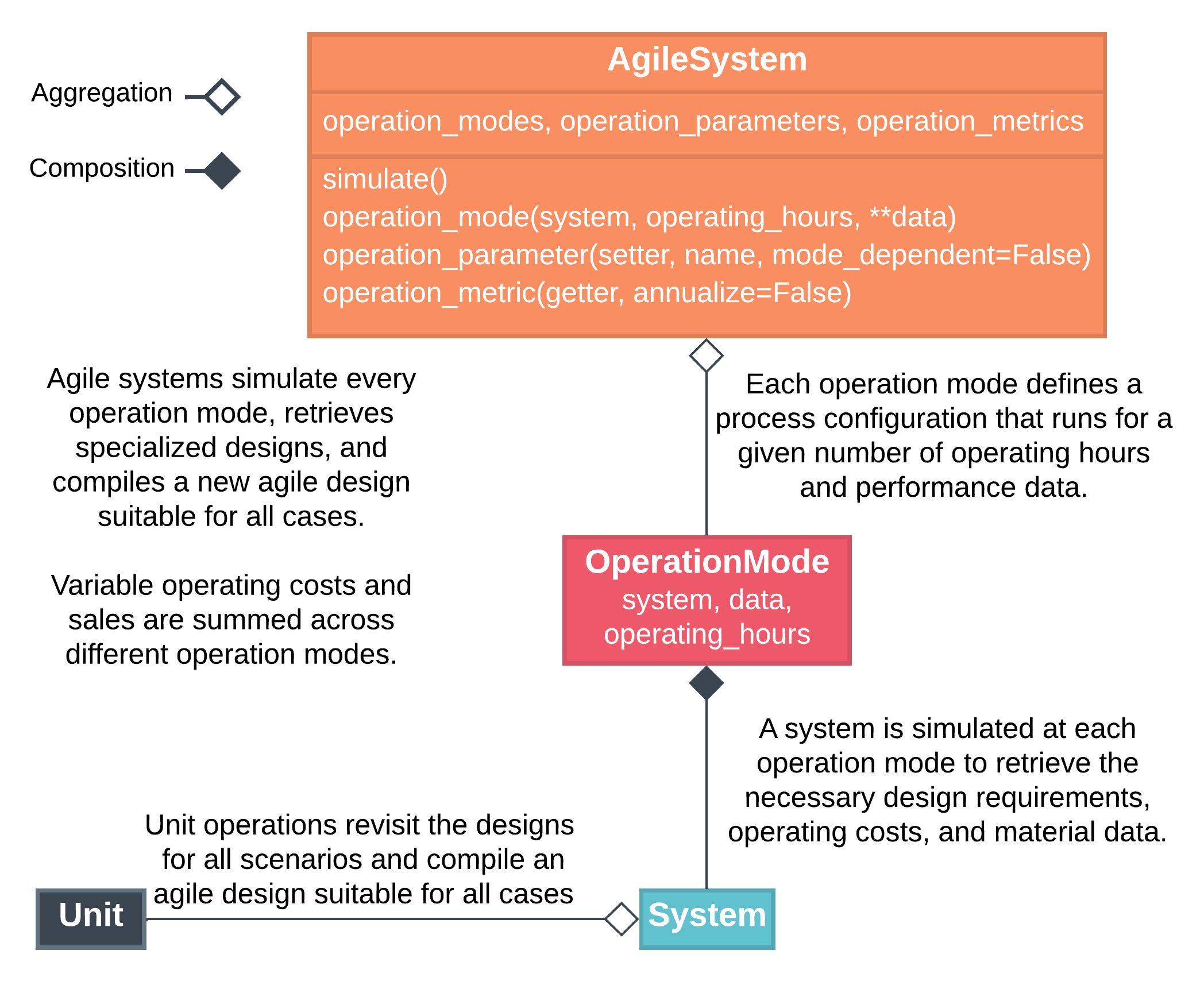
BioSTEAM is able to conservatively design operationally flexible biorefineries that can switch configurations, vary feedstocks, and even vary operating conditions throughout the year. Switching operation modes throughout the year is modeled using an AgileSystem object, which simulates each mode of operation and compiles new agile designs for each unit operation suitable for all operation modes. For example, an agile distillation column would have the largest diameter and number of operating stages required among all operation modes. Each operation mode runs for a defined number of operating hours, allowing the variable operating costs (e.g. material and utility costs) and sales to be summed across different operation modes. This preliminary agile design assumption leads to conservative estimates around utility costs as some units may be over-designed. For example, a distillation column with a higher number of stages will require a lower reflux ratio and less utilities to reach a target separation. The following UML diagram summarizes how BioSTEAM agile biorefinery models work:

19.2. Agile sugarcane and sweet sorghum biorefinery#

One drawback of processing sugarcane is its short harvesting period of 4-5 months in southern USA, which limits biorefinery operations to 5-7 months a year. Because sweet sorghum can be harvested when sugarcane is not in season, an idle sugarcane biorefinery could potentially increase biofuel production by processing sorghum. A logistics study accounting for cropland and harvesting by Cutz et al. proposed that sugarcane plants may potentially process sweet sorghum at least 1 month before, and 1 month after the sugarcane season [1]. The co-utilization of sugarcane and sorghum feedstocks has been achieved at an industrial-scale trial in Zimbabwe, which demonstrated that sweet sorghum can be processed without any modifications to an existing sugarcane mill [2].

Here we model an agile sugcarcane/sorghum biorefinery using an AgileSystem object. We use two operation modes, one for sugarcane and one for sorghum. As an example, we expose fermentation efficiency as an operation parameter and set different efficiencies for each operation mode. We also define the emissions as a metric and view both annualized and detailed results by operation mode:

[1]:

import biosteam as bst
from warnings import filterwarnings; filterwarnings('ignore')
from biorefineries import sugarcane as sc

# Create the agile system object
agile_sys = bst.AgileSystem()

# Create sugarcane system
sc.load()
sugarcane_sys = sc.sugarcane_sys

# Create new soghum system; which is exactly the same as sugarcane but with a different feedstock.
# Systems remember the configuration they had when they were created, which makes it
# possible to change configurations without affecting old systems.
sugarcane = sc.U101.ins[0]
sc.U101.ins[0] = None # Remove stream without warnings
sc.U101.ins[0] = sorghum = bst.Stream(
    'sorghum',
    Water=0.7,
    Glucose=0.0111,
    Sucrose=0.126,
    Ash=0.006,
    Cellulose=0.0668,
    Hemicellulose=0.0394,
    Lignin=0.0358,
    Solids=0.015,
    total_flow=333334,
    price=sc.sugarcane.price,
    units='kg/hr',
)
sorghum_sys = bst.System.from_units('sorghum_sys', sugarcane_sys.units)

# Define operation parameters.
@agile_sys.operation_parameter
def set_fermentation_efficiency(X):
    sc.R301.X = X

# If mode dependent, the mode is also passed to the setter when the agile system is simulated.
@agile_sys.operation_parameter(mode_dependent=True)
def set_feedstock_flow_rate(flow_rate, mode):
    # We can define a "feedstock" attribute later.
    mode.feedstock.F_mass = flow_rate

# Define operation metrics
# If annualized, the metric returns the integral sum across operation hours.
# In other words, the result of this metric will be in ton / yr (instead of ton / hr).
@agile_sys.operation_metric(annualize=True)
def net_emissions(mode):
    return (sc.R301.outs[0].imass['CO2'] + sc.BT.outs[0].imass['CO2']) / 907.18

# When metric is not annualized, the metric returns a dictionary of results by
# operation mode (in ton / hr).
@agile_sys.operation_metric
def emissions_by_mode(mode):
    return (sc.R301.outs[0].imass['CO2'] + sc.BT.outs[0].imass['CO2']) / 907.18

# Note how the name of the parameter defaults to the name used in the function (e.g., X, flow_rate).
sugarcane_mode = agile_sys.operation_mode(
    system=sugarcane_sys, operating_hours=24*200, X=0.90, feedstock=sugarcane,
    flow_rate=333334,
)

# Assume fermentation of sorghum is less efficient for demonstration purposes.
# Assume a similar flow rate is available for sorghum.
sorghum_mode = agile_sys.operation_mode(
    system=sorghum_sys, operating_hours=24*60, X=0.85, feedstock=sorghum,
    flow_rate=330000,
)

Note how the operation modes we defined are stored in the AgileSystem object:

[2]:

agile_sys.operation_modes

[2]:

[OperationMode(system=sugarcane_sys, operating_hours=4800, X=0.9, feedstock=sugarcane, flow_rate=333334),
 OperationMode(system=sorghum_sys, operating_hours=1440, X=0.85, feedstock=sorghum, flow_rate=330000)]

Simulate and retrieve general system results:

[3]:

agile_sys.simulate()
print(f'Sales: {agile_sys.sales / 1e6:.0f} MMUSD/yr')
print(f'Material cost: {agile_sys.material_cost / 1e6:.0f} MMUSD/yr')
print(f'Utility cost: {agile_sys.utility_cost / 1e6:.0f} MMUSD/yr')

Sales: 112 MMUSD/yr
Material cost: 74 MMUSD/yr
Utility cost: -23 MMUSD/yr

Retrieve annualized and non-annualized emissions:

[4]:

print(f'Net emissions: {net_emissions():.0f} ton/yr')
print('Emissions by mode:')
for mode, value in emissions_by_mode().items():
    print(f" {mode.system}: {value:.0f} ton/hr")

Net emissions: 702716 ton/yr
Emissions by mode:
 sugarcane_sys: 112 ton/hr
 sorghum_sys: 116 ton/hr

Just like BioSTEAM System objects, summarized power and heat utilities for agile systems. These have been averaged across operation modes on an hourly basis:

[5]:

agile_sys.power_utility

PowerUtility:
 consumption: 8.35e+03 kW
 production: 7.09e+04 kW
 power: -6.26e+04 kW
 cost: -4.07e+03 USD/hr

We can create a new TEA object with the agile system to see how our IRR has changed:

[6]:

sugarcane_mode.simulate()
sc.sugarcane_tea.IRR = sc.sugarcane_tea.solve_IRR()
print('Sugarcane only')
print(f'NPV: {round(sc.sugarcane_tea.NPV/1e6)} MMUSD')
print(f'IRR: {sc.sugarcane_tea.IRR:.0%}')
print(f'TCI: {sc.sugarcane_tea.TCI/1e6:.0f} MMUSD')

# Recreate the TEA object using the agile system
agile_tea = sc.ConventionalEthanolTEA(
    system=agile_sys,
    IRR=0.15,
    duration=(2018, 2038),
    depreciation='MACRS7',
    income_tax=0.35,
    operating_days=260, # Total sum of operating days across operation modes
    lang_factor=3,
    construction_schedule=(0.4, 0.6),
    WC_over_FCI=0.05,
    labor_cost=2.5e6,
    fringe_benefits=0.4,
    property_tax=0.001,
    property_insurance=0.005,
    supplies=0.20,
    maintenance=0.01,
    administration=0.005
)
agile_sys.simulate()
agile_tea.IRR = agile_tea.solve_IRR()
print()
print('Agile Sugarcane/Sorghum')
print(f'NPV: {round(agile_tea.NPV/1e6)} MMUSD')
print(f'IRR: {agile_tea.IRR:.0%}')
print(f'TCI: {agile_tea.TCI/1e6:.0f} MMUSD')

Sugarcane only
NPV: 0 MMUSD
IRR: 14%
TCI: 207 MMUSD

Agile Sugarcane/Sorghum
NPV: 0 MMUSD
IRR: 18%
TCI: 216 MMUSD

While the IRR is higher due to increased production, note how the capital cost increases slightly due to the different feedstock composition and operation.

19.2.1. References#

Cutz, L.; Sanchez-Delgado, S.; Ruiz-Rivas, U.; Santana, D. Bioenergy Production in Central America: Integration of Sweet Sorghum into Sugar Mills. Renewable and Sustainable Energy Reviews 2013, 25, 529–542. https://doi.org/10.1016/j.rser.2013.05.007.
Woods, J. The Potential for Energy Production Using Sweet Sorghum in Southern Africa. Energy for Sustainable Development 2001, 5 (1), 31–38. https://doi.org/10.1016/S0973-0826(09)60018-1.

[ ]: