19. Uncertainty and sensitivity#
TEA/LCA is a powerful tool to understand the potential sustainability of a technology. But it can be extremely difficult to navigate uncertainties in design decisions (e.g., refinery size and location), market variability, and technological performance. Evaluating just one representative scenario (under a single set of assumptions) gives an incomplete picture that is not conclusive. This is especially true for conceptual and early-stage technologies, which have higher levels of uncertainty. We need to pair TEA/LCA with rigorous uncertainty/sensitivity analyses to explore the landscape of potential outcomes, identify representative scenarios (through sensitivity analysis), and establish technological performance targets. To learn more about expediting RD&D through modeling, we recommend reading on quantitive sustainable design (QSD) methodology.


As one of its central features, BioSTEAM streamlines TEA/LCA with rigorous uncertainty/sensitivity analyses to empower researchers with the ability to navigate uncertainty and guide RD&D. Using NREL’s model for cellulosic ethanol production from cornstover as a conceptual case study, this tutorial will demonstrate how to construct a model and perform Monte Carlo-based uncertainty/sensitivity analyses to establish potential targets for improvement.
19.1. Framework#
BioSTEAM streamlines uncertainty analysis with an object-oriented framework where a Model object samples from parameter distributions and evaluates sustainability indicators at each new condition. In essence, a Model object sets parameter values, simulates the biorefinery system, and evaluates indicators across an array of samples.
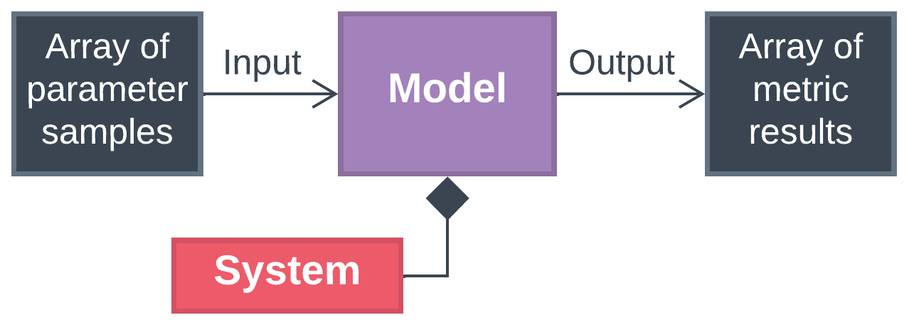
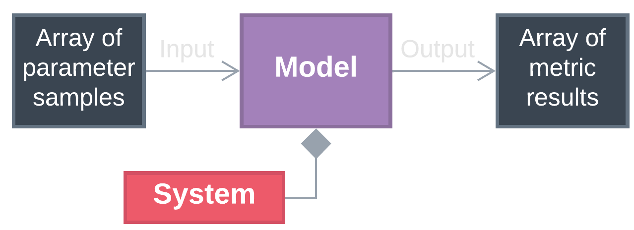
On the backend, Model objects cut down simulation time using a number of strategies, including sorting the samples to minimize perturbations to the system between simulation.
19.1.1. Probability distributions#
Let’s first learn how to create common parameter distributions using chaospy.
A triangular distribution is typically used when the input parameter is uncertain within given limits, but is heuristically known to take a particular value. Create a triangular distribution:
[1]:
from warnings import filterwarnings; filterwarnings('ignore')
from chaospy import distributions as shape
lower_bound = 0
most_probable = 0.5
upper_bound = 1
triang = shape.Triangle(lower_bound, most_probable, upper_bound)
print(triang)
Triangle(0, 0.5, 1)
A uniform distribution is used when the theoretical limits of the parameter is known, but no information is available to discern which values are more probable. Create a uniform distribution:
[2]:
from chaospy import distributions as shape
lower_bound = 0
upper_bound = 1
unif = shape.Uniform(lower_bound, upper_bound)
print(unif)
Uniform()
A large set of distributions are available through chaospy, but generally triangular and uniform distributions are the most widely used to describe the uncertainty of parameters in Monte Carlo analyses.
19.1.2. Input parameters and sustainability indicators#
Parameter and Indicator objects are simply structures BioSTEAM uses to set input parameters and evaluate sustainability/performance indicators.
Parameter objects use a setter function to set the parameter value related to an element (e.g. unit operation, stream, etc.). They can have a distribution (e.g., triangular, uniform) attribute for Model objects to sample from. Parameters also have name, units of measure, and baseline value attributes for bookkeeping purposes. BioSTEAM incorporates the element, name, and units of measure when creating a DataFrame of Monte Carlo results and parameter
distributions. Similarly, an Indicator object uses a getter function for to evaluate the indicator value and has name, element, and units of measure attributes for bookkeeping.
Hopefully things will be become clearer with the following examples using a cellulosic ethanol production process.
19.2. Creating a Model object#
Model objects are used to evaluate indicators given a set of system parameters.
Create a Model object of the cellulosic ethanol:
[3]:
import biosteam as bst
from biorefineries import cellulosic
from biorefineries.tea import create_cellulosic_ethanol_tea
bst.nbtutorial()
chemicals = cellulosic.create_cellulosic_ethanol_chemicals()
bst.settings.set_thermo(chemicals)
cellulosic.load_process_settings()
bst.F.set_flowsheet('cellulosic_ethanol') # F is the main flowsheet
system = cellulosic.create_cellulosic_ethanol_system()
tea = create_cellulosic_ethanol_tea(system)
model = bst.Model(system)
The Model object begins with no parameters and no indicators:
[4]:
model
Model:
parameters: None
indicators: None
19.2.1. Add sustainability/performance indicators#
[5]:
@model.indicator(units='USD/kg')
def MESP(): return tea.solve_price(bst.F.ethanol)

@model.indicator(units='10^6 * USD')
def TCI(): return tea.TCI / 1e6 # total capital investment

model
Model:
parameters: None
indicators: MESP [USD/kg]
            TCI [10^6 * USD]
Note that the decorator uses the function to create an Indicator object and adds it to the model.
19.2.2. Add input parameters#
[6]:
fermentation = bst.F.R303
ethanol_rxn = fermentation.cofermentation[0]
xylose_rxn = fermentation.cofermentation[4]
@model.parameter(
    element='fermentation', units='% theoretical', # Metadata (does not affect simulation)
    bounds=(85, 95), # Lower and upper bound
    distribution='uniform', # Same as shape.Uniform(lower, upper)
    baseline=0.5 * (80 + 95), # Baseline assumption
    coupled=True, # Optional, tells BioSTEAM this impacts mass/energy balances
)
def set_glucose_to_ethanol_yield(glucose_to_ethanol_yield):
    ethanol_rxn.X = glucose_to_ethanol_yield / 100

@model.parameter(
    element='fermentation', units='% theoretical',
    bounds=(70, 90), # Baseline defaults to the average of the lower and upper bounds.
    distribution='uniform',
    coupled=True,
)
def set_xylose_to_ethanol_yield(xylose_to_ethanol_yield):
    xylose_rxn.X = xylose_to_ethanol_yield / 100

feedstock = bst.F.cornstover # The feedstock stream
lb = feedstock.price * 0.9 # Minimum price
ub = feedstock.price * 1.1 # Maximum price
@model.parameter(
    element='cornstover', units='USD/kg',
    bounds=(lb, ub),
    baseline=feedstock.price,
    distribution='triangular' # Defaults to shape.Triangular(lower=lb, midpoint=baseline, upper=ub)
)
def set_feed_price(feedstock_price):
    feedstock.price = feedstock_price

processing_capacity = feedstock.F_mass * tea.operating_hours / 1e3 # Annual processing capacity MT / y
lb = processing_capacity * 0.9
ub = processing_capacity * 1.1
@model.parameter(
    units='MT/yr',
    bounds=(lb, ub),
    element='Biorefinery',
    baseline=processing_capacity,
    distribution='triangular',
    coupled=True,
)
def set_processing_capacity(processing_capacity):
    feedstock.F_mass = 1e3 * processing_capacity / tea.operating_hours

model
Model:
parameters: Fermentation - Glucose to ethanol yield [% theoretical]
            Fermentation - Xylose to ethanol yield [% theoretical]
            Cornstover - Feedstock price [USD/kg]
            Biorefinery - Processing capacity [MT/yr]
indicators: MESP [USD/kg]
            TCI [10^6 * USD]
Note that the model.parameter decorator uses the function to create a Parameter object and adds it to the model.
19.2.3. Overview of the model#
Get dictionary that contain DataFrame objects of parameter distributions:
[7]:
df_dct = model.get_distribution_summary()
df_dct['Uniform']
[7]:
| Element | Name | Units | Shape | lower | upper | |
|---|---|---|---|---|---|---|
| 0 | fermentation | Glucose to ethanol yield | % theoretical | Uniform | 85 | 95 |
| 1 | fermentation | Xylose to ethanol yield | % theoretical | Uniform | 70 | 90 |
[8]:
df_dct['Triangle']
[8]:
| Element | Name | Units | Shape | lower | midpoint | upper | |
|---|---|---|---|---|---|---|---|
| 0 | cornstover | Feedstock price | USD/kg | Triangle | 0.0464 | 0.0516 | 0.0567 |
| 1 | Biorefinery | Processing capacity | MT/yr | Triangle | 7.89e+05 | 8.77e+05 | 9.64e+05 |
Evaluate baseline scenario:
[9]:
baseline_scenario = model.get_baseline_scenario()
baseline_scenario
| fermentation | Glucose to ethanol yield [% theoretical] | 87.5 |
|---|---|---|
| Xylose to ethanol yield [% theoretical] | 80 | |
| cornstover | Feedstock price [USD/kg] | 0.0516 |
| Biorefinery | Processing capacity [MT/yr] | 8.77e+05 |
[10]:
model(baseline_scenario)
| - | MESP [USD/kg] | 0.72 |
|---|---|---|
| TCI [10^6 * USD] | 382 |
19.2.4. Monte Carlo uncertainty analysis#
Sample from a joint distribution, and simulate samples:
[11]:
import numpy as np
N_samples = 200
rule = 'L' # For Latin-Hypercube sampling
np.random.seed(1234) # For consistent results
samples = model.sample(N_samples, rule)
model.load_samples(samples, sort=True)
model.exception_hook = 'raise'
model.evaluate(
    notify=100 # Also print elapsed time after 50 simulations
)
[100] Elapsed time: 11 sec
[200] Elapsed time: 22 sec
All data from simulation is stored in <Model>.table:
[12]:
full_problem_space = model.table.copy() # All evaluations are stored as a pandas DataFrame
full_problem_space
[12]:
| Element | fermentation | cornstover | Biorefinery | - | ||
|---|---|---|---|---|---|---|
| Feature | Glucose to ethanol yield [% theoretical] | Xylose to ethanol yield [% theoretical] | Feedstock price [USD/kg] | Processing capacity [MT/yr] | MESP [USD/kg] | TCI [10^6 * USD] |
| 0 | 85.4 | 79.2 | 0.0523 | 9.05e+05 | 0.726 | 390 |
| 1 | 85.1 | 73.7 | 0.0491 | 8.47e+05 | 0.728 | 376 |
| 2 | 86.8 | 71.6 | 0.0538 | 8.21e+05 | 0.759 | 369 |
| 3 | 87.8 | 87 | 0.0548 | 8.99e+05 | 0.721 | 386 |
| 4 | 88.4 | 74.2 | 0.0504 | 8.15e+05 | 0.731 | 366 |
| ... | ... | ... | ... | ... | ... | ... |
| 195 | 92.1 | 86.4 | 0.0481 | 8.36e+05 | 0.687 | 367 |
| 196 | 85.3 | 79.9 | 0.0533 | 9.07e+05 | 0.73 | 391 |
| 197 | 90.4 | 86.1 | 0.0479 | 8.39e+05 | 0.69 | 369 |
| 198 | 93.1 | 80.4 | 0.0523 | 8.6e+05 | 0.709 | 375 |
| 199 | 89.7 | 84.7 | 0.0532 | 8.47e+05 | 0.719 | 371 |
200 rows × 6 columns
Create a kernel density scatter plot to visualize the two economic indicators under uncertainty:
[13]:
import thermosteam as tmo
import matplotlib.pyplot as plt
format_units = tmo.units_of_measure.format_units
ylabel = f"MESP [{format_units('USD/kg')}]"
xlabel = f"TCI [{format_units('10^6 USD')}]"
def plot_uncertainty(table): # This function will be useful later
    fig, ax, axes = bst.plots.plot_kde(
        y=table[MESP.index],
        x=table[TCI.index],
        ylabel=ylabel,
        xlabel=xlabel,
        aspect_ratio=1.1,
    )
plot_uncertainty(model.table)

Note that the brighter areas signify that scenario results are more clustered and hence, more probable.
19.3. Sensitivity with Spearman’s rank order correlation#
Model objects also presents methods for sensitivity analysis such as Spearman’s correlation, a measure of monotonicity between variables:
[14]:
df_rho, df_p = model.spearman_r()
print(df_rho['-', 'MESP [USD/kg]'])
Element       Parameter
fermentation  Glucose to ethanol yield [% theoretical]   -0.512
              Xylose to ethanol yield [% theoretical]    -0.636
cornstover    Feedstock price [USD/kg]                    0.603
Biorefinery   Processing capacity [MT/yr]                -0.208
Name: (-, MESP [USD/kg]), dtype: float64
Create a tornado plot of Spearman’s correlation between all parameters and IRR:
[15]:
bst.plots.plot_spearman_1d(df_rho['-', 'MESP [USD/kg]'],
                           index=[i.describe() for i in model.parameters],
                           name='MESP [USD/kg]')
[15]:
(<Figure size 1920x1440 with 3 Axes>,
 <Axes: xlabel="Spearman's correlation with MESP [USD/kg]">)

19.4. Single point sensitivity#
A quick way to evaluate sentivity is through single point sensitivity analysis, whereby a metric is evaluated at the baseline and at the lower and upper limits of each parameter. This method ignores the interactions between parameters and their distributions, but can help screen whether a system is sensitive to a given parameter. Model objects also facilitate this analysis:
[16]:
baseline, lower, upper = model.single_point_sensitivity()
print('BASELINE')
print('--------')
print(baseline)
print()
print('LOWER')
print('-----')
print(lower)
print()
print('UPPER')
print('-----')
print(upper)
BASELINE
--------
Element  Feature
-        MESP [USD/kg]      0.72
         TCI [10^6 * USD]    382
dtype: float64

LOWER
-----
Element                                                      -
Feature                                          MESP [USD/kg] TCI [10^6 * USD]
Element      Feature
fermentation Glucose to ethanol yield [% theo...         0.727              383
             Xylose to ethanol yield [% theor...         0.736              384
cornstover   Feedstock price [USD/kg]                    0.693              382
Biorefinery  Processing capacity [MT/yr]                 0.735              358

UPPER
-----
Element                                                      -
Feature                                          MESP [USD/kg] TCI [10^6 * USD]
Element      Feature
fermentation Glucose to ethanol yield [% theo...         0.699              378
             Xylose to ethanol yield [% theor...         0.704              379
cornstover   Feedstock price [USD/kg]                    0.746              382
Biorefinery  Processing capacity [MT/yr]                 0.707              405
Create a tornado plot of the lower and upper values of the IRR:
[17]:
IRR, utility_cost = model.indicators
metric_index = IRR.index
index = [i.describe(distribution=False) # Instead of displaying distribution, it displays lower, baseline, and upper values
         for i in model.parameters]
bst.plots.plot_single_point_sensitivity(100 * baseline[metric_index],
                                        100 * lower[metric_index],
                                        100 * upper[metric_index],
                                        name='MESP [USD/kg]',
                                        index=index)
[17]:
(<Figure size 1920x1440 with 3 Axes>, <Axes: xlabel='MESP [USD/kg]'>)

Note that blue represents the upper limit while red the lower limit. Also note that local sensitivity (as estimated by the single point sensitivity analysis) is different from the global sensitivity (estimated by Spearman’s rank order correlation coefficient of Monte Carlo results).
19.5. Scenario analysis#
Let’s have a look at two different potential scenarios: a conservative and a prospective “improved” fermentation performance.
[18]:
set_glucose_to_ethanol_yield.active = False
set_xylose_to_ethanol_yield.active = False
set_glucose_to_ethanol_yield(85)
set_xylose_to_ethanol_yield(80)
model.evaluate() # Reevaluate at the conservative scenario sub-space
conservative_scenario_subspace = model.table.copy()
set_glucose_to_ethanol_yield(95)
set_xylose_to_ethanol_yield(90)
model.evaluate() # Reevaluate at the prospective scenario sub-space
prospective_scenario_subspace = model.table.copy()
[19]:
scenarios = [
    'full problem space',
    'conservative scenario sub-space',
    'prospective scenario sub-space',
]
data = [
    full_problem_space,
    conservative_scenario_subspace,
    prospective_scenario_subspace,
]
dct = bst.plots.plot_montecarlo(
    data=np.array([i[MESP.index] for i in data]),
    xmarks=[i.replace(' ', '\n') for i in scenarios]
)
plt.ylabel(ylabel)
[19]:
Text(0, 0.5, 'MESP [$\\mathrm{USD} \\cdot \\mathrm{kg}^{-1}$]')

Note how the targeted improvements to fermentation can benefit economic outcomes. We can also directly compare these key scenario sub-spaces under harmonized assumptions on price and processing capacity.
[20]:
improvement = prospective_scenario_subspace - conservative_scenario_subspace
fig, ax, axes = bst.plots.plot_kde(
    y=improvement[MESP.index],
    x=improvement[TCI.index],
    ylabel='$\Delta$' + ylabel,
    xlabel='$\Delta$' + xlabel,
    aspect_ratio=1.1,
)

Note how the prospective scenario subspace leads to lower MESP and TCI compared to the convervative scenario subspace.