15. Thermodynamic engine#
15.1. Pure component chemical models#
BioSTEAM’s thermodynamic engine is called ThermoSTEAM. It packages chemical and mixture thermodynamic models in a flexible framework that allows users to fully customize and extend the models, as well as create new models. Central to all thermodynamic algorithms is the Chemical object, which contain the same thermodynamic models and data as thermo’s Chemical objects, but present an API more suitable for BioSTEAM’s needs.
[1]:
import biosteam as bst # Imports everything in thermosteam too
bst.nbtutorial()
# Initialize chemical with an identifier (e.g. by name, CAS, InChI...)
Water = bst.Chemical('Water')
Water.show()
Chemical: Water (phase_ref='l')
[Names]  CAS: 7732-18-5
         InChI: H2O/h1H2
         InChI_key: XLYOFNOQVPJJNP-U...
         common_name: water
         iupac_name: ('oxidane',)
         pubchemid: 962
         smiles: O
         formula: H2O
[Groups] Dortmund: <1H2O>
         UNIFAC: <1H2O>
         PSRK: <1H2O>
         NIST: <Empty>
[Data]   MW: 18.015 g/mol
         Tm: 273.15 K
         Tb: 373.12 K
         Tt: 273.16 K
         Tc: 647.1 K
         Pt: 611.65 Pa
         Pc: 2.2064e+07 Pa
         Vc: 5.5948e-05 m^3/mol
         Hf: -2.8582e+05 J/mol
         S0: 70 J/K/mol
         LHV: -44011 J/mol
         HHV: -0 J/mol
         Hfus: 6010 J/mol
         Sfus: None
         omega: 0.3443
         dipole: 1.85 Debye
         similarity_variable: 0.16653
         iscyclic_aliphatic: 0
         combustion: {'H2O': 1.0}
Access pure component data:
[2]:
# CAS number
Water.CAS
[2]:
'7732-18-5'
[3]:
# Molecular weight (g/mol)
Water.MW
[3]:
18.01528
[4]:
# Boiling point (K)
Water.Tb
[4]:
373.124295848
Temperature (in Kelvin) and pressure (in Pascal) dependent properties can be computed:
[5]:
# Vapor pressure (Pa)
Water.Psat(T=373.15)
[5]:
101417.99665995422
[6]:
# Surface tension (N/m)
Water.sigma(T=298.15)
[6]:
0.07197220523022962
[7]:
# Liquid molar volume (m^3/mol)
Water.V(phase='l', T=298.15, P=101325)
[7]:
1.8068319928499427e-05
[8]:
# Vapor molar volume (m^3/mol)
Water.V(phase='g', T=298.15, P=101325)
[8]:
0.02350635143332423
[9]:
# With user-specified units of measure:
Water.get_property('rho', 'kg/m3', phase='l', T=298.15, P=101325)
[9]:
997.0644792261086
Temperature dependent properties are managed by objects:
[10]:
Water.Psat
[10]:
VaporPressure(CASRN="7732-18-5", Tb=373.124295848, Tc=647.096, Pc=22064000.0, omega=0.3443, extrapolation="AntoineAB|DIPPR101_ABC", method="IAPWS_PSAT", Tmin=235.0, Tmax=647.096)
Phase dependent properties have attributes with model handles for each phase:
[11]:
Water.V
PhaseTPHandle(phase, T, P=None) -> V [m^3/mol]
[12]:
Water.V.l
[12]:
VolumeLiquid(CASRN="7732-18-5", MW=18.01528, Tb=373.124295848, Tc=647.096, Pc=22064000.0, Vc=5.59480372671e-05, Zc=0.22943845208106295, omega=0.3443, dipole=1.85, Psat=VaporPressure(CASRN="7732-18-5", Tb=373.124295848, Tc=647.096, Pc=22064000.0, omega=0.3443, extrapolation="AntoineAB|DIPPR101_ABC", method="IAPWS_PSAT", Tmin=235.0, Tmax=647.096), extrapolation="constant", method="HEOS_FIT", method_P="COSTALD_COMPRESSED", tabular_extrapolation_permitted=True, Tmin=251.165, Tmax=582.3864)
A new model can be added easily using add_method, for example:
[13]:
def User_antoine_model(T):
     return 10.0**(10.116 -  1687.537 / (T - 42.98))
Water.Psat.add_method(f=User_antoine_model, Tmin=273.20, Tmax=473.20)
Water.Psat.method
[13]:
'USER_METHOD'
The add_method method is a high level interface that even lets you create a constant model:
[14]:
Water.Cn.l.add_method(75.31)
Water.Cn('l', 350)
[14]:
75.31
Choose what model to use through the method attribute:
[15]:
Water.Cn.l.all_methods
[15]:
{'COOLPROP',
 'CRCSTD',
 'DADGOSTAR_SHAW',
 'HEOS_FIT',
 'JANAF',
 'POLING_CONST',
 'ROWLINSON_BONDI',
 'ROWLINSON_POLING',
 'USER_METHOD',
 'WEBBOOK_SHOMATE',
 'ZABRANSKY_SPLINE_C',
 'ZABRANSKY_SPLINE_C_1',
 'ZABRANSKY_SPLINE_C_2',
 'ZABRANSKY_SPLINE_C_3',
 'ZABRANSKY_SPLINE_C_4'}
[16]:
Water.Cn.l.method = 'ZABRANSKY_SPLINE_C'
Water.Cn('l', 350)
[16]:
75.6223925836403
15.2. Managing chemical sets#
Define multiple chemicals as a Chemicals object:
[17]:
chemicals = bst.Chemicals(['Water', 'Ethanol'])
chemicals
Chemicals([Water, Ethanol])
The chemicals are attributes:
[18]:
(chemicals.Water, chemicals.Ethanol)
[18]:
(Chemical('Water'), Chemical('Ethanol'))
Chemicals are indexable:
[19]:
Water = chemicals['Water']
print(repr(Water))
Chemical('Water')
[20]:
chemicals['Ethanol', 'Water']
[20]:
[Chemical('Ethanol'), Chemical('Water')]
Chemicals are also iterable:
[21]:
for chemical in chemicals:
    print(repr(chemical))
Chemical('Water')
Chemical('Ethanol')
More chemicals can also be appended:
[22]:
Propanol = bst.Chemical('Propanol')
chemicals.append(Propanol)
chemicals
Chemicals([Water, Ethanol, Propanol])
The main benefit of using a Chemicals object, is that they can be compiled and used as part of a thermodynamic property package, as defined through a Thermo object:
[23]:
# A Thermo object is built with an iterable of Chemicals or their IDs.
# Default mixture, thermodynamic equilibrium models are selected.
thermo = bst.Thermo(chemicals)
thermo.show()
Thermo(
    chemicals=CompiledChemicals([Water, Ethanol, Propanol]),
    mixture=IdealMixture(...
        include_excess_energies=False
    ),
    Gamma=DortmundActivityCoefficients,
    Phi=IdealFugacityCoefficients,
    PCF=MockPoyintingCorrectionFactors
)
Creating a thermo property package, may be a little challenging if some chemicals cannot be found in the database, in which case they can be built from scratch. A complete example on how this can be done is available in another tutorial.
15.3. Material and energy balances#
A Stream object is the main interface for estimating thermodynamic properties, vapor-liquid equilibrium, and material and energy balances. First set the thermo property package and we can start creating streams:
[24]:
# This also works: tmo.settings.set_thermo(['Water', 'Ethanol', 'Propanol'])
bst.settings.set_thermo(thermo)
s1 = bst.Stream(Water=20, Ethanol=20, units='kg/hr')
s1.show(flow='kg/hr')
Stream: s1
phase: 'l', T: 298.15 K, P: 101325 Pa
flow (kg/hr): Water    20
              Ethanol  20
Create another stream at a higher temperature:
[25]:
s2 = bst.Stream(Water=10, units='kg/hr', T=350, P=101325)
s2.show(flow='kg/hr')
Stream: s2
phase: 'l', T: 350 K, P: 101325 Pa
flow (kg/hr): Water  10
Mix both streams into a new one:
[26]:
s_mix = bst.Stream()
s_mix.mix_from([s1, s2])
s_mix.show(flow='kg/hr')
Stream: s_mix
phase: 'l', T: 310.54 K, P: 101325 Pa
flow (kg/hr): Water    30
              Ethanol  20
Check the energy balance through enthalpy:
[27]:
s_mix.H - (s1.H + s2.H)
[27]:
-5.884430720470846e-10
Note that the balance is not perfect as the solver stops within a small temperature tolerance. However, the approximation is less than 0.01% off:
[28]:
error = s_mix.H - (s1.H + s2.H)
percent_error = 100 * error / (s1.H + s2.H)
print(f"{percent_error:.2%}")
-0.00%
Split the mixture to two streams by defining the component splits:
[29]:
# First define an array of component splits
component_splits = s_mix.chemicals.array(['Water', 'Ethanol'], [0, 1])
s_mix.split_to(s1, s2, component_splits)
s1.T = s2.T = s_mix.T # Take care of energy balance
s1.show(flow='kg/hr')
s2.show(flow='kg/hr')
Stream: s1
phase: 'l', T: 310.54 K, P: 101325 Pa
flow (kg/hr): Ethanol  20
Stream: s2
phase: 'l', T: 310.54 K, P: 101325 Pa
flow (kg/hr): Water  30
Separate out stream from mixture:
[30]:
s_mix.separate_out(s2)
s_mix.show(flow='kg/hr') # Only enthanol will remain
Stream: s_mix
phase: 'l', T: 310.54 K, P: 101325 Pa
flow (kg/hr): Ethanol  20
Note that the energy balance still holds:
[31]:
error = s_mix.H - s1.H
percent_error = 100 * error / s2.H
print(f"{percent_error:.2%}")
0.00%
15.4. Flow rates#
The most convenient way to get and set flow rates is through the get_flow and set_flow methods:
[32]:
# Set and get flow of a single chemical
# in gallons per minute
s1.set_flow(1, 'gpm', 'Water')
s1.get_flow('gpm', 'Water')
[32]:
1.0
[33]:
# Set and get flows of many chemicals
# in kilograms per hour
s1.set_flow([10, 20], 'kg/hr', ('Ethanol', 'Water'))
s1.get_flow('kg/hr', ('Ethanol', 'Water'))
[33]:
array([10., 20.])
It is also possible to index flow rate data using chemical IDs through the imol, imass, and ivol indexers:
[34]:
s1.imol.show()
ChemicalMolarFlowIndexer (kmol/hr):
(l) Water    1.11
    Ethanol  0.217
[35]:
s1.imol['Water']
[35]:
1.1101687012358397
[36]:
s1.imol['Ethanol', 'Water']
[36]:
array([0.217, 1.11 ])
All flow rates are stored as a sparse array in the mol attribute. These arrays work just like numpy arrays, but are more scalable (saving memory and increasing speed) for sparse chemical data:
[37]:
s1.mol # Molar flow rates [kmol/hr]
[37]:
sparse([1.11 , 0.217, 0. ])
Mass and volumetric flow rates are also available for convenience:
[38]:
s1.mass
[38]:
sparse([20., 10., 0.])
[39]:
s1.vol
[39]:
sparse([0.02 , 0.013, 0. ])
The data of these arrays are linked to the molar flows:
[40]:
# Mass flows are always up to date with molar flows
s1.mol[0] = 1
s1.mass[0]
[40]:
18.01528
[41]:
# Changing mass flows changes molar flows
s1.mass[0] *= 2
s1.mol[0]
[41]:
2.0
[42]:
# New arrays are not linked to molar flows
s1.mass + 2 # A new array is created
[42]:
sparse([38.031, 12. , 2. ])
[43]:
# Array methods are also the same
s1.mass.mean()
[43]:
15.34352
15.5. Thermal condition#
Temperature and pressure can be get and set through the T and P attributes:
[44]:
s1.T = 400.
s1.P = 2 * 101325.
s1.show()
Stream: s1
phase: 'l', T: 400 K, P: 202650 Pa
flow (kmol/hr): Water    2
                Ethanol  0.217
The phase may also be changed (‘s’ for solid, ‘l’ for liquid, and ‘g’ for gas):
[45]:
s1.phase = 'g'
Notice that VLE is not enforced, but it is possible to perform. For now, just check that the dew point is lower than the actual temperature to assert it must be gas:
[46]:
dp = s1.dew_point_at_P() # Dew point at constant pressure
dp
[46]:
DewPointValues(T=390.81, P=202650, IDs=('Water', 'Ethanol'), z=[0.902 0.098], x=[0.991 0.009])
[47]:
dp.T < s1.T
[47]:
True
It is also possible to get and set in other units of measure:
[48]:
s1.set_property('P', 1, 'atm')
s1.get_property('P', 'atm')
[48]:
1.0
[49]:
s1.set_property('T', 125, 'degC')
s1.get_property('T', 'degF')
[49]:
256.99999999999994
Enthalpy and entropy can also be set. In both cases, an energy balance is made to solve for temperature at isobaric conditions:
[50]:
s1.H = 1.05 * s1.H
s1.get_property('T', 'degC') # Temperature should go up
[50]:
184.9588719718261
[51]:
s1.S = 0.95 * s1.S
s1.get_property('T', 'degC') # Temperature should go down
[51]:
74.98140649417905
15.6. Thermal properties#
Thermodynamic properties are pressure, temperature and phase dependent. In the following examples, let’s just use water as it is easier to check properties:
[52]:
s_water = bst.Stream(Water=1, units='kg/hr')
s_water.rho # Density [kg/m^3]
[52]:
997.0644792261086
[53]:
s_water.T = 350
s_water.rho # Density changes
[53]:
973.7419512246709
Get properties in different units:
[54]:
s_water.get_property('sigma', 'N/m') # Surface tension
[54]:
0.06324769600985489
[55]:
s_water.get_property('V', 'm3/kmol') # Molar volume
[55]:
0.01850108232200766
15.7. Flow properties#
Several flow properties are available, such as net material and energy flow rates:
[56]:
# Net molar flow rate [kmol/hr]
s_water.F_mol
[56]:
0.05550843506179199
[57]:
# Net mass flow rate [kg/hr]
s_water.F_mass
[57]:
1.0
[58]:
# Net volumetric flow rate [m3/hr]
s_water.F_vol
[58]:
0.00102696612664403
[59]:
# Enthalpy flow rate [kJ/hr]
s_water.H
[59]:
216.91884940751328
[60]:
# Entropy flow rate [kJ/hr]
s_water.S
[60]:
4.556326412564778
[61]:
# Capacity flow rate [J/K]
s_water.C
[61]:
4.194462916586701
15.8. Phase equilibrium#
When streams are created, by default, they do not perform phase equilibrium. To perform phase equilibrium assuming 2 liquid phases and 1 gas phase is possible (i.e., vapor-liquid-liquid equilibrium), pass vlle=True:
[62]:
bst.settings.set_thermo(['Water', 'Ethanol', 'Octane'])
s = bst.Stream(Water=1, Ethanol=0.2, Octane=2, T=358, P=101325,
               phase='l', # Guess phase
               vlle=True)
s.show() # Notice how 3 phases co-exist
MultiStream: s
phases: ('L', 'g', 'l'), T: 358 K, P: 101325 Pa
flow (kmol/hr): (L) Water    0.0995
                    Ethanol  0.0381
                    Octane   1.8
                (g) Water    0.424
                    Ethanol  0.146
                    Octane   0.199
                (l) Water    0.476
                    Ethanol  0.0155
                    Octane   4.15e-05
For certain mixtures, we can be sure that 3 phases cannot co-exist and it is more efficient to assume 2 phases instead when estimating equilibrium. Before moving into equilibrium calculations, it may be useful to have a look at the phase envelopes to understand chemical interactions and ultimately how they partition between phases.
Plot the binary phase evelope of two chemicals in vapor-liquid equilibrium at constant pressure:
[63]:
import matplotlib.pyplot as plt
eq = bst.equilibrium # Thermosteam's equilibrium module
eq.plot_vle_binary_phase_envelope(['Ethanol', 'Water'], P=101325)
plt.show()

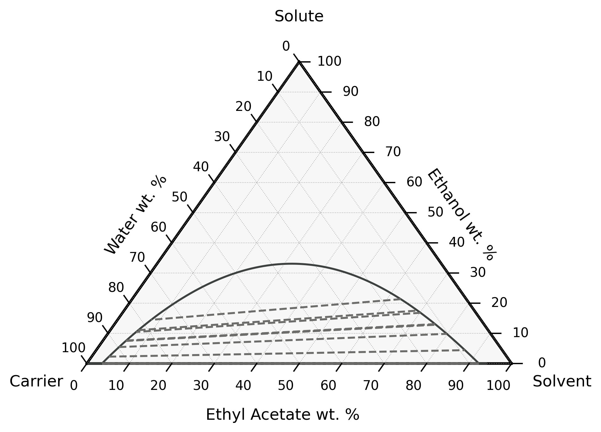
Plot the ternary phase diagram of three chemicals in liquid-liquid equilibrium at constant pressure:
[64]:
# You'll need to "pip install python-ternary" to run this line
bst.settings.set_thermo(['Water', 'Ethanol', 'EthylAcetate'])
eq.plot_lle_ternary_diagram(carrier='Water', solute='Ethanol', solvent='EthylAcetate', T=298.15)
plt.show()
15.9. Vapor-liquid equilibrium#
Vapor-liquid equilibrium can be performed by setting 2 degrees of freedom from the following list: T (Temperature; in K), P (Pressure; in Pa), V (Vapor fraction), H (Enthalpy; in kJ/hr), and S (Entropy; in kJ/K/hr).
For example, set vapor fraction and pressure:
[65]:
s_eq = bst.Stream(Water=10, Ethanol=10)
s_eq.vle(V=0.5, P=101325)
s_eq.show(composition=True)
MultiStream: s_eq
phases: ('g', 'l'), T: 353.94 K, P: 101325 Pa
composition (%): (g) Water    38.7
                     Ethanol  61.3
                     -------  10 kmol/hr
                 (l) Water    61.3
                     Ethanol  38.7
                     -------  10 kmol/hr
Note that the stream is now a MultiStream to manage multiple phases. Each phase can be accessed separately too:
[66]:
s_eq['l'].show()
Stream:
phase: 'l', T: 353.94 K, P: 101325 Pa
flow (kmol/hr): Water    6.13
                Ethanol  3.87
[67]:
s_eq['g'].show()
Stream:
phase: 'g', T: 353.94 K, P: 101325 Pa
flow (kmol/hr): Water    3.87
                Ethanol  6.13
Note that the phase of these substreams cannot be changed:
[68]:
with bst.print_error: s_eq['g'].phase = 'l'
AttributeError: phase is locked
Again, the most convenient way to get and set flow rates is through the get_flow and set_flow methods:
[69]:
# Set flow of liquid water
s_eq.set_flow(1, 'gpm', ('l', 'Water'))
s_eq.get_flow('gpm', ('l', 'Water'))
[69]:
1.0
[70]:
# Set multiple liquid flows
key = ('l', ('Ethanol', 'Water'))
s_eq.set_flow([10, 20], 'kg/hr', key)
s_eq.get_flow('kg/hr', key)
[70]:
array([10., 20.])
Chemical flows across all phases can be retrieved if no phase is given:
[71]:
# Get water and ethanol flows summed across all phases
s_eq.get_flow('kg/hr', ('Water', 'Ethanol'))
[71]:
array([ 89.791, 292.216])
However, setting chemical data of MultiStream objects requires the phase to be specified:
[72]:
with bst.print_error: s_eq.set_flow([10, 20], 'kg/hr', ('Water', 'Ethanol'))
IndexError: multiple phases present; must include phase key to set chemical data
Similar to Stream objects, all flow rates can be accessed through the imol, imass, and ivol attributes:
[73]:
s_eq.imol # Molar flow rates
MolarFlowIndexer (kmol/hr):
(g) Water         3.87
    Ethanol       6.13
(l) Water         1.11
    Ethanol       0.217
[74]:
# Index a single chemical in the liquid phase
s_eq.imol['l', 'Water']
[74]:
1.1101687012358397
[75]:
# Index multiple chemicals in the liquid phase
s_eq.imol['l', ('Ethanol', 'Water')]
[75]:
array([0.217, 1.11 ])
[76]:
# Index the vapor phase
s_eq.imol['g']
[76]:
sparse([3.874, 6.126, 0. ])
[77]:
# Index flow of chemicals summed across all phases
s_eq.imol['Ethanol', 'Water']
[77]:
array([6.343, 4.984])
Because multiple phases are present, overall chemical flows in MultiStream objects cannot be set like in Stream objects:
[78]:
with bst.print_error: s_eq.imol['Ethanol', 'Water'] = [1, 0]
IndexError: multiple phases present; must include phase key to set chemical data
Chemical flows must be set by phase:
[79]:
s_eq.imol['l', ('Ethanol', 'Water')] = [1, 0]
One main difference between a MultiStream object and a Stream object is that the mol attribute no longer stores any data, it simply returns the total flow rate of each chemical. Setting an element of the array raises an error to prevent the wrong assumption that the data is linked:
[80]:
s_eq.mol
[80]:
sparse([3.874, 7.126, 0. ])
[81]:
with bst.print_error: s_eq.mol[0] = 1
ValueError: assignment destination is read-only
Note that for both Stream and MultiStream objects, get_flow, imol, and mol return chemical flows across all phases when given only chemical IDs.
15.10. Liquid-liquid equilibrium#
Liquid-liquid equilibrium (LLE) only requires the temperature. Pressure is not a significant variable as liquid fungacity coefficients are not a strong function of pressure.
[82]:
bst.settings.set_thermo(['Water', 'Butanol', 'Octane'])
liquid_mixture = bst.Stream(Water=100, Octane=100, Butanol=5)
liquid_mixture.lle(T=300)
liquid_mixture.show()
MultiStream: liquid_mixture
phases: ('L', 'l'), T: 300 K, P: 101325 Pa
flow (kmol/hr): (L) Water    98.5
                    Butanol  1.21
                    Octane   0.00198
                (l) Water    1.46
                    Butanol  3.79
                    Octane   100
15.11. Vapor-liquid-liquid equilibrium#
Vapor-liquid-liquid equilibrium can be performed by setting 2 degrees of freedom from the following list: T (Temperature; in K), P (Pressure; in Pa), V (Vapor fraction), H (Enthalpy; in kJ/hr), and S (Entropy; in kJ/K/hr).
[83]:
bst.settings.set_thermo(['Water', 'Ethanol', 'Octane'])
mixture = bst.Stream(Water=100, Octane=40, Ethanol=5)
mixture.vlle(V=0.1, P=101325)
mixture.show()
MultiStream: mixture
phases: ('L', 'g', 'l'), T: 358.97 K, P: 101325 Pa
flow (kmol/hr): (L) Water    89.6
                    Ethanol  2.16
                    Octane   0.00669
                (g) Water    8.36
                    Ethanol  2.25
                    Octane   3.89
                (l) Water    2
                    Ethanol  0.588
                    Octane   36.1
[84]:
mixture.vapor_fraction
[84]:
0.10000045858254801
Warning
VLLE is an experimental feature; results may not be accurate nor consistent.